Wireless Sensor Network, 2009, 1, 284-292
doi:10.4236/wsn.2009.14035 Published Online November 2009 (http://www.scirp.org/journal/wsn).
The Estimation of Radial Exponential Random
Vectors in Additive White Gaussian Noise
P. Kittisuwan1, S. Marukatat2, W. Asdornwised1
1Department of Electrical Engineering, Faculty of Engineering,
Chulalongkorn University, Bangkok, Thailand
2Image Laboratory, National Electronics and Computer Technology Center (NECTEC), Thailand
Received April 22, 2009; revised June 15, 2009; accepted J un e 22, 2009
Abstract
Image signals are always disturbed by noise during their transmission, such as in mobile or network commu-
nication. The received image quality is significantly influenced by noise. Thus, image signal denoising is an
indispensable step during image processing. As we all know, most commonly used methods of image de-
noising is Bayesian wavelet transform estimators. The Performance of various estimators, such as maximum
a posteriori (MAP), or minimum mean square error (MMSE) is strongly dependent on correctness of the
proposed model for original data distribution. Therefore, the selection of a proper model for distribution of
wavelet coefficients is important in wavelet-based image denoising. This paper presents a new image de-
noising algorithm based on the modeling of wavelet coefficients in each subband with multivariate Radial
Exponential probability density function (PDF) with local variances. Generally these multivariate extensions
do not result in a closed form expression, and the solution requires numerical solutions. However, we drive a
closed form MMSE shrinkage functions for a Radial Exponential random vectors in additive white Gaussian
noise (AWGN). The estimator is motivated and tested on the problem of wavelet-based image denoising. In
the last, proposed, the same idea is applied to the dual-tree complex wavelet transform (DT-CWT), This
Transform is an over-complete wavelet transform.
Keywords: MMSE Estimator, Radial Exponential Random Vectors, Wavelet Transform, Image Denoising
1. Introduction
The denoising of a natural image corrupted by Gaussian
noise is a classic problem in signal processing. The distor-
tion of images by noise is common during its, acquisition,
processing, compression, mobile and network transmis-
sion. Traditional algorithms perform image denoising
based on threshold function methods, such as soft-thresh-
old and hard-threshold [1]. If the wavelet transform and
MMSE estimator are used for this problem, the solution
requires a priori knowledge about wavelet coefficients.
Therefore, two problems arise: 1) what kinds of distribu-
tions represent the wavelet coefficients? 2) What is the
corresponding estimator (shrinkage function)?
Figure 1 illustrates the histogram of photographic
image and PDF plots. The PDF plots illustrate the mar-
ginal Radial Exponential PDF and Gaussian PDF. The
histogram in Figure 1 is very symmetric with zero mean
and the histogram of wavelet coefficients are more like
marginal Radial Exponential PDF, it is more peaked and
the tails are heavier, than the Gaussian distribution.
It is known that the amplitude of wavelet coefficients
tend to propagate across scales. This parent-child relation
is also underlined by the empirical joint histogram be-
tween parent and child coefficients as shown in [2]. In [3],
they developed a multivariate spherically contoured
Laplacian density that is similar to the Radial Exponential
random vectors in its function form, but the marginal of
Laplacian random vectors are not Radial Exponential den-
sity. Indeed, Radial Exponential random vectors specialize
to Laplacian random vectors in the scalar case


1d

. In
this paper we focus on Radial Exponential random vectors
with local variances to model these locality and persis-
tence properties of wavelet coefficients. The rest of this
paper is organized as follows. In Section 2, the basic idea
of Bayesian denoising will be briefly described. Subsec-
tion 2.1 describes wavelet coefficients model, these mod-
ls try to capture the dependencies between a coeffi- e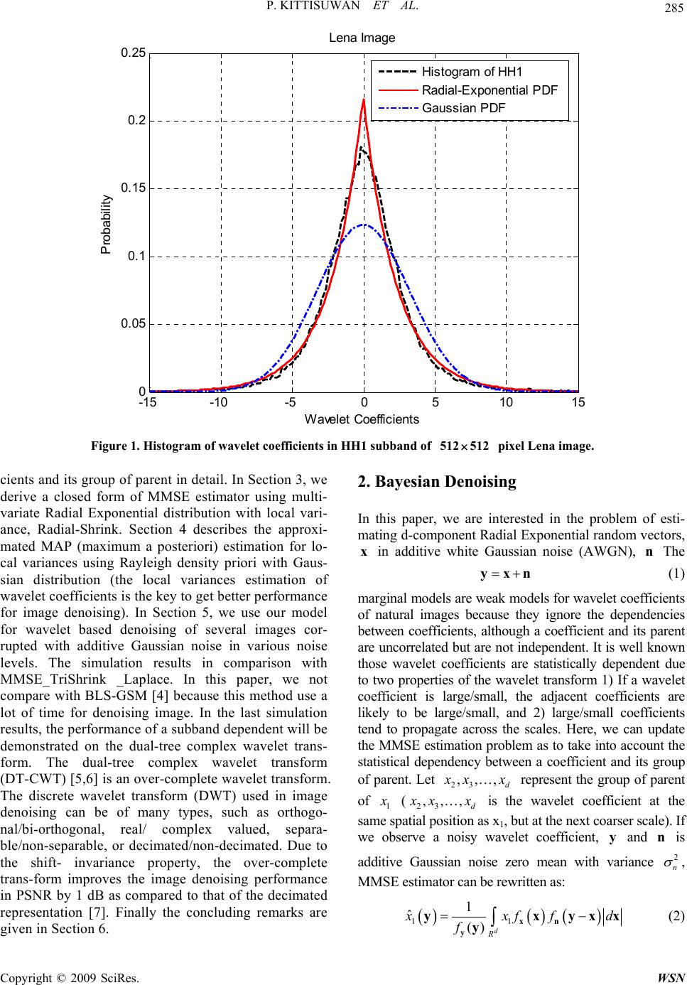

P. KITTISUWAN ET AL.
285
-15 -10-5 05 10 15
0
0.05
0.1
0.15
0.2
0.25
Wa vel e t Co e ffic ien ts
Probability
Lena Image
Histogram of HH1
Radial -Exponential PDF
Gaussi an P DF
Figure 1. Histogram of wavelet c oefficients in HH1 subband of 512512

pixel Lena image.
cients and its group of parent in detail. In Section 3, we
derive a closed form of MMSE estimator using multi-
variate Radial Exponential distribution with local vari-
ance, Radial-Shrink. Section 4 describes the approxi-
mated MAP (maximum a posteriori) estimation for lo-
cal variances using Rayleigh density priori with Gaus-
sian distribution (the local variances estimation of
wavelet coefficients is the key to get better performance
for image denoising). In Section 5, we use our model
for wavelet based denoising of several images cor-
rupted with additive Gaussian noise in various noise
levels. The simulation results in comparison with
MMSE_TriShrink _Laplace. In this paper, we not
compare with BLS-GSM [4] because this method use a
lot of time for denoising image. In the last simulation
results, the performance of a subband dependent will be
demonstrated on the dual-tree complex wavelet trans-
form. The dual-tree complex wavelet transform
(DT-CWT) [5,6] is an over-complete wavelet transform.
The discrete wavelet transform (DWT) used in image
denoising can be of many types, such as orthogo-
nal/bi-orthogonal, real/ complex valued, separa-
ble/non-separable, or decimated/non-decimated. Due to
the shift- invariance property, the over-complete
trans-form improves the image denoising performance
in PSNR by 1 dB as compared to that of the decimated
representation [7]. Finally the concluding remarks are
given in Section 6.
2. Bayesian Denoising
In this paper, we are interested in the problem of esti-
mating d-component Radial Exponential random vectors,
in additive white Gaussian noise (AWGN), The
x n


y
xn (1)
marginal models are weak models for wavelet coefficients
of natural images because they ignore the dependencies
between coefficients, although a coefficient and its parent
are uncorrelated but are not independent. It is well known
those wavelet coefficients are statistically dependent due
to two properties of the wavelet transform 1) If a wavelet
coefficient is large/small, the adjacent coefficients are
likely to be large/small, and 2) large/small coefficients
tend to propagate across the scales. Here, we can update
the MMSE estimation problem as to take into account the
statistical dependency between a coefficient and its group
of parent. Let 23 ,,,
d
x
xx represent the group of parent
of 1
x
(23 ,,,
d
x
xx is the wavelet coefficient at the
same spatial position as x1, but at the next coarser scale). If
we observe a noisy wavelet coefficient, and is
additive Gaussian noise zero mean with variance ,
MMSE estimator can be rewritten as:
y n

2
n
  
11
1
ˆ()d
R
x
xf fd
f

xn
y
y
x
y
xx
y (2)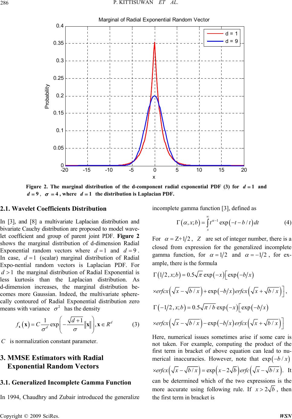

P. KITTISUWAN ET AL.
286
-20 -15 -10 -5 0510 1520
0
0.05
0.1
0.15
0.2
0.25
0.3
0.35
0.4
x
Probability
Margi nal of Radial E xponent i al Random V ector
d = 1
d = 9
Figure 2. The marginal distribution of the d-component radial exponential PDF (3) for and
,
1d
9d24

, where the distribution is Laplacian PDF. 1d
2.1. Wavelet Coefficients Distribution
In [3], and [8] a multivariate Laplacian distribution and
bivariate Cauchy distribution are proposed to model wave-
let coefficient and group of parent joint PDF. Figure 2
shows the marginal distribution of d-dimension Radial
Exponential random vectors where and 1d9d

.
In case, (scalar) marginal distribution of Radial
Expo-nential random vectors is Laplacian PDF. For
the marginal distribution of Radial Exponential is
less kurtosis than the Laplacian distribution. As
d-dimension increases, the marginal distribution be-
comes more Gaussian. Indeed, the multivariate sphere-
cally contoured of Radial Exponential distribution zero
means with variance
1d
1d
2

has the density

11
exp, d
d
d
f
CR
 






xxx
x
(3)
C is normalization constant parameter.
3. MMSE Estimators with Radial
Exponential Random Vectors
3.1. Generalized Incomplete Gamma Function
In 1994, Chaudhry and Zubair introduced the generalize
incomplete gamma function [3], defined as
 
1
,;exp /
x
x
bt tbtd



 
t (4)
For Ζ+12


,
Z
are set of integer number, there is a
closed from expression for the generalized incomplete
gamma function, for 12


and 12


la
, for ex-
ample, there is the formu




12, ;0.5expexp
x
bx    
bx




/exp /erfcxxb xbxerfcxxb x  
,






12, ;0.5/expexp
x
bbx 

 
 bx





/exp /erfcxxb xbxerfcxxb x  

Here, numerical issues sometimes arise if some care is
not taken. For example, computing the product of the
first term in bracket of above equation can lead to nu-
merical inaccuracies. However, note that


exp /bx






/exp2 /erfcx xbxxberfc xbx .
If
It
can be determined which of the two expressions is the
more accurate using following rule. 2
x
b, then
the first term in bracket

is

P. KITTISUWAN ET AL.
287


exp// .bxerfcxxbx

Other cases, the first
term in the bracket is

exp 2
x
b

/erfcxb x.
Indeed, the generalized incomplete gamma function sat-
isfies a recurrence relation for computing its values for
other order,

from [9,10]

1
( 1,;)1,;,;

x
bxb
b



xb

 
exp/ .
x
xbx



 (5)
3.2. MMSE Estimator with Multivariate Radial
Exponential D is t r i b u t i on
Multivariate spherically contoured of Radial Exponential
density can be generated by
x
zxs,
where is d-component zero mean iid Gaussian ran-
dom vectors with variance
s
2



2
22
2
1exp 2
2d
f







s
s
s
and is a gamma PDF .
The two distribution are iid. Setting
z() 4exp(2)
z
fz zz,0z
az

, then
. Changing the random variable of
asx


,,zasx.
Using Jacobian transform

21d
J
aa, then the PDF
of random vectors is given by x


2
0
z
f
Jf afda
a




xs
x
x

2
0
1
2z
d
afaf
a a
 
 
 
sxda (6)
From MMSE estimator (2), we would like to find
()fy
y
and
 
d
R
A
ff d
xn
xyxx. If the noise sig-
nal is independent additive white Gaussian noise
(AWGN) with variance
n
2
n

,


2
22
2
1exp 2
2dn
n
f







n
n
n
First, the PDF of is given by the multivariate
convolution. The multivariate convolution defines as:
y
()() ()
d
R
f
ff d

yxn
yxyxx (7)
Using (6) gives



2
0
1
2
dz
d
R
fafafdaf
a a


 


 
 


ys
x
yyd
n
xx


2
0
1
2
d
zd
R
af affdda
a a













 sn
xyx x
Using Gaussian convolution formula [3]

1
dd
R
ff d
a a





sn
xyxx



2
22
22 2
22 2
11
exp
2
2dd
n
na
a








y
Therefore,




2
22
22 2
0
11
2
2
zdd
n
fafa a







yy

2
22 2
exp
2n
da
a










y
 

3
2
222 2
0
2
2
22 2
8
2
exp 22
d
d
n
n
a
a
ad
a











ya
Changing the variable of integration, using
222
22, 4
n
t adt ada  ,
gives



22
2
2
exp 2n
d
f




yy


2
2
2 22
22
2
2exp
n
n
d
ttd
tt









yt

Using the generalized incomplete gamma function in
(4), we get


2
22 2
222 2
exp 22
()2 ,;
2 ()
nn
d
d
f
 
 






y
y
y
2
22
22
22
1, ;
2
nn
d 






y
2

(8)

288 P. KITTISUWAN ET AL.
Second, from MMSE estimator (2), we would like to
find
() ()
di
R
A
xf fd
xn
xyxx
Using (6) gives
A


2
0
1
2(
diz
d
R
)
x
afafdaf d
a a


 

 
 

 sn
xyxx

2
0
1
2(
d
zi
d
R
af axffdda
a a








 sn
xyx x)
Using Gaussian convolution formula [3]

1
did
R
xf fd
a a
 


sn
xyxx




2
22
2
22 222 2
22 2
1exp
2
2
id
n
n
ya
a
a

 







y
n
a



Therefore,




22
2
2
22 222 2
0
1
2
2
i
zd
nn
ya
Aafa
aa

 




2
22 2
exp
2n
da
a 






y


52
21
222 2
0
8
2
id
d
n
ay
a







2
2
22 2
exp 2
2n
ad
a 






ya
Changing the variable of integration at


22
2
2
4exp 2ni
d
y
A





2
2
2
42222 2
21 2
2
4
exp
n
nn
d
tt td
tt


 



 




y
t

Using the generalized incomplete gamma function in
(4), we get

2 22 2
222 2
exp 22
2, ;
2
()
ni n
d
yd
A
 
 



 

y
2
22
22 2 2
2222 2
42 2
1, ;4, ;
22
nn n n
dd

 



2












yy

(9)
Solving (2) using (8) and (9) gives the MMSE estima-
tor,
2
2
22
2
ˆ2, ;
2
n
ii d
xy








y
2
22
2222
2222 2
22
22 2
22 222
42 2
1, ;4, ;
22
22 2
2, ;1, ;
22
nn n n
nn n
dd
dd
  
 
 
 



2













 
 




yy
yy





Setting3d

and using thce relation of gen-
er comp
e recurren
alized inlete gamma function (5), we get

22
22
11 22
2
42
1
ˆ1,
2
nn
xy







 






y
y
2
;

22
222
22 22
2
242
1,;
2
nnn














y
y



32 2
22
122 2
2
2
22
222
22 222
22
exp 2
222 11
,; ,;
22
nn
n
nnn




 












 




  


 


y
y
yy
(10)
We called this method Radial-Shrink.
. Parameter Estimation
o apply our estimator, we need to know noise variance
4
T
2
n

and the variance of noise-free 2

. To estimate
e variance from noisy wavelet coefients, a robust
median estimator is used from the 1
nois fic
H
H subband [11].
2
1
2()
ˆ0.6745
n
median HH





(11)
Under the assumption that marginal variance in wave-
let child coefficient is difference for each data point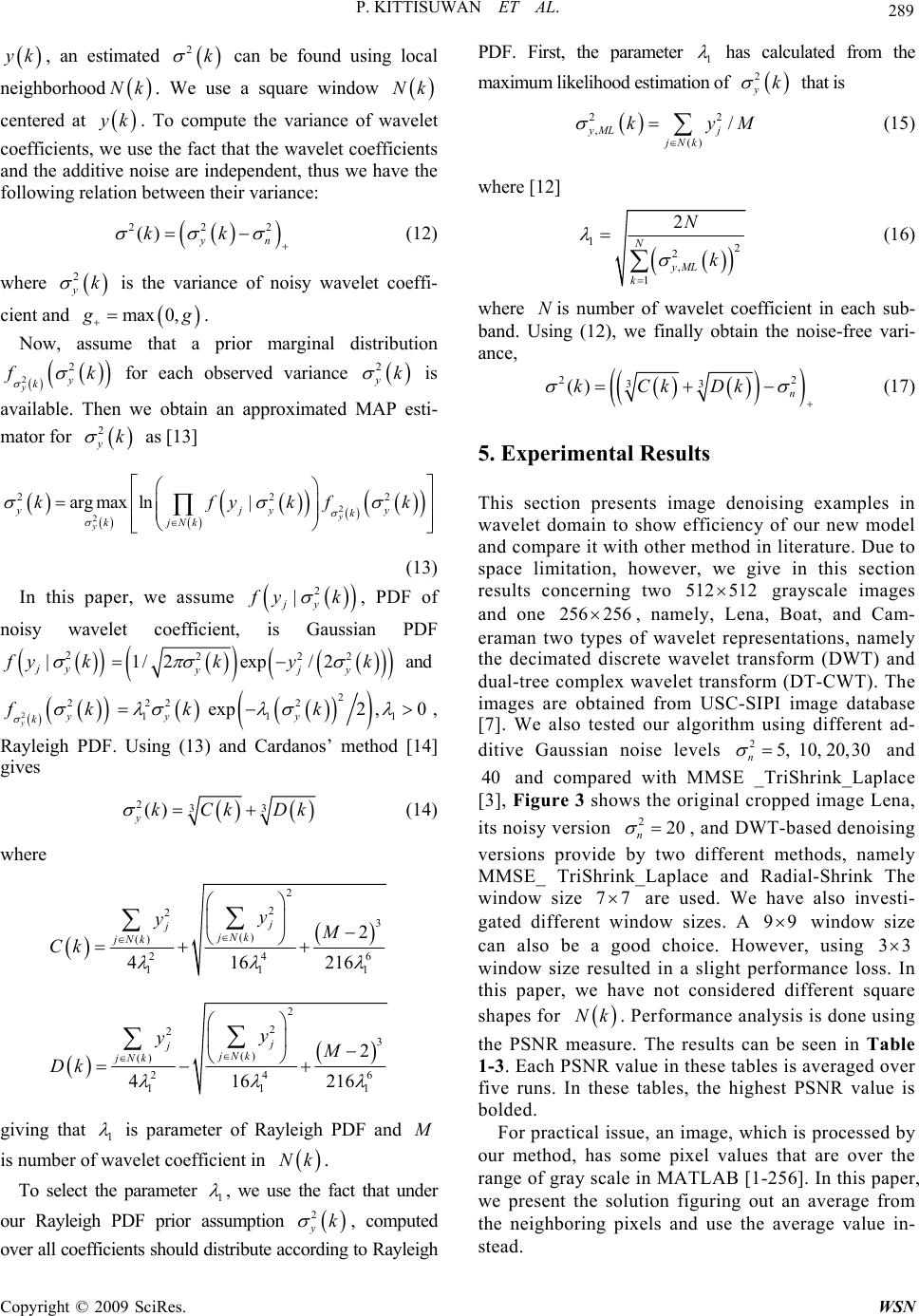

P. KITTISUWAN ET AL.
289

y
k, an estimated

2k
 can be found using local
ne borhood

Nk. Wee a square window igh us


Nk
centered at

y
k. To compute the variance of w
coefficients, we use the fact that the wavelet coefficients
and the additive noise are independent, thus we have the
following relation between their variance:


222
() yn kk 


avelet
(12)
where is the variance of no

2
yk

d
isy wavelet coeffi-
cient an

max 0,
g
g.
Now, assume that a prior marginal distribution

2



2
yy
k

f
k

for each observed variance 


2

AP e
yk is
we obtain an approximated Msti-
y

available. Then
mator for 2k 

as [13]
2
y
k 
(13)
In this paper, we assum




 

 2
2
22
arg maxln|y
y
yjy
k
jNk k
kfykf













e


2
|
jy
f
yk  , PDF of
noisy wavelet coefficient, is Gaussian PDF


2
|
jy
f
yk 








22
1/ 2e
yj
k k   and
2
xp/2y y 


2
yy
k

2
f
k

22
k  




1y


2
2
exp2 ,0k   ,
[14]
11y

Rayleigh PDF. Using (13) and Cardanos’ method
gives

233
()
ykCkDk
  (14)
where
 
2
2
23
()
()
24
11
2
416 216
j
jjNk
jNk
y
yM
Ck







 


6
1

 
2
2
23
()
()
24
11
2
416216
j
jjNk
jNk
y
yM
Dk 6
1








 


giving that 1

is parameter of Rayleigh PDF and
M
is number of wavelet coefficient in
he

Nk.
To select t parameter 1

, we use the fact that un
our Rayleigh PDF prior assumptiok
der
n computed
over all coefficients should distribute according to Rayleigh
PD

2
y
 ,
F. First, the parameter 1

has calculated from the
maximum likelihood estimation of

2
yk
 t is

tha


22
,
(
/
yML j
jNk
kyM 


)

(15)
where [12]


12
co
2
,
1
2
N
yM
k





(16)
where is number of wat
band. Using (12), we finall obtain
ance,
L
N
k
vele
y
Nefficient in each sub-
the noise-free vari-
 




22
33
() n kCkDk 

 (17)
5. Experimental Results
his section presents imagxamples in
ieur new model
ace limitation, however, wethis section
Te denoising e
ncy of o
give in
wavelet domain to show effic
and compare it with other method in literature. Due to
sp
results concerning two 512 512 grayscale images
and one 256256

, namely, Lena, Boat, and Cam-
eraman two types of wavelet representations, namely
the decimated discrete wavelet transform (DWT) and
dual-tree complex wavelet transform (DT-CWT). The
images are obtained from USC-SIPI image database
[7]. We also tested our algorithm using different ad-
ditive Gaussian noise levels 25,10,20, 30
n
  and
40 and compared with MMSE _TriShrink_Laplace
[3], Figure 3 shows the original cropped image Lena,
its noisy version 220
n
 , and Dising
sions provide by two different methods, namely
MMSE_ TriShrink_Laplace and Radial-Shrink The
window size 77
WT-based deno
ver

are used. We have also investi-
gated different window sizes. A 99 window size
can also be a good choice. However, using 33

window size resulted in a slight performance loss. In
this paper, we have not considered different square
shapes for


Nk. Performance analysis is done using
the PSNR measure. The results can be seen in Table
1-3. Each PSNR value in these tables is averaged over
five runs. In te e tables, the highest PSNR value is
bolded.
For practical issue, an image, which is processed by
our method, has some pixel values that are over the
range of gray scale in MATLAB [1-256]. In this paper,
we prese
h s
nt the solution figuring out an average from
the neighboring pixels and use the average value in-
stead.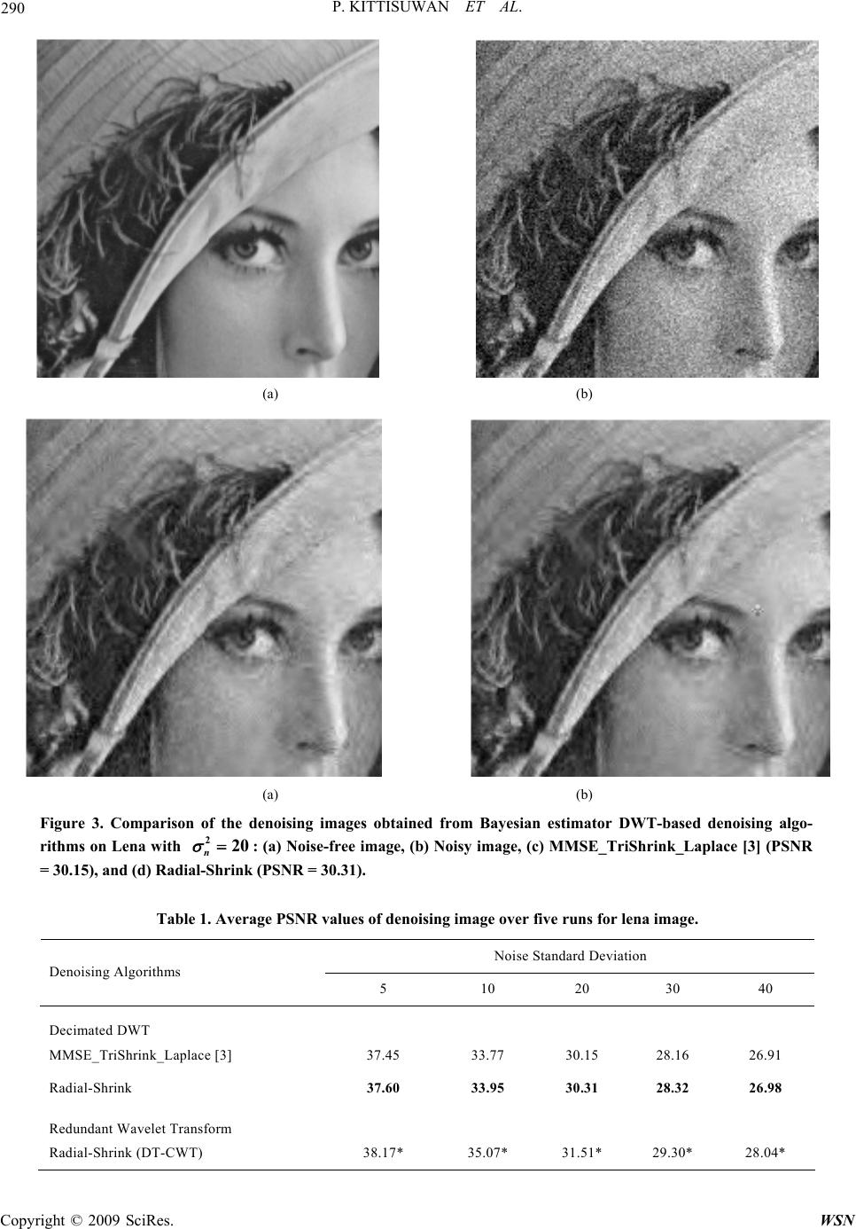

P. KITTISUWAN ET AL.
290
(a) (b)
(a) (b)
Figure 3. Comparison of the denoising images obtained from Bayesian estimator DWT-based denoising algo-
rithms on Lena with TriShrink_Laplace [3] (PSNR
image over five runs for lena image.
220

n: (a) Noise-free image, (b) Noisy image, (c) MMSE_
= 30.15), and (d) Radial-Shrink (PSNR = 30.31).
Table 1. Average PSNR values of denoising
Noise Standard Deviation
Denoising Algori
5 1030 40
thms
20
Decimated DWT
MMSE_TriShrink_Laplace [3] 37.45 33.77 30.15 28.16 26.91
elet Transform
Radial-Shrink (DT-CWT) 38.17* 35.07* 31.51* 29.30* 28.04*
Radial-Shrink 37.60 33.95 30.31 28.32 26.98
Redundant Wav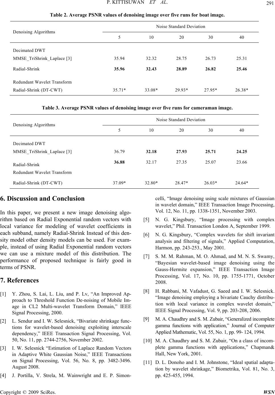

P. KITTISUWAN ET AL.
291
Table 2. Average PSNR values of denoising image over five runs for boat image.
tandation Noise Sard Devi
Denoisin
40
g Algorithms
5 10 20 30
Decimated DWT
MMSE_TriShrink_Laplace [3] 35 3 2 2 2
35.96 32.43 28.89 26.82 25.46
DT-CWT)
.942.328.75 6.735.31
Radial-Shrink
Redundant Wavelet Transform
Radial-Shrink (35.71* 33.08* 29.93* 27.95* 26.38*
e PSNR values of denoising image over five rueram
Noise Standard Deviation
Table 3. Averagns for caman image.
Denoising Algo
40
rithms
5 10 20 30
Decimated DWT
MMSE_TriShrink_Laplace [3] 36 3 2 2 2
36.88 32.17 27.35 25.07 23.66
DT-CWT)
.79 2.187.93 5.714.25
Radial-Shrink
Redundant Wavelet Transform
Radial-Shrink (37.09* 32.80* 28.47* 26.03* 24.64*
6. Discussion and Conc
this paper, we present a new image denoising algo-
ndom vectors with
cal variance for modeling of wavelet coefficients in
Lai, L. Liu, and P. Lv, “An Improved Ap-
shold Function De-noising of Mobile Im-
ulti-wavelet Transform Domain,” IEEE
action Signal Processing, Vol.
3482-3496.
celli, “Image denoising using scale mixtures of Gaussian
waveln,” IEsactionProcessing,
Vol. 12, No. 11, pp. 1338-1351, November 2003.
Transaction London A, September 1999.
wamy,
d and I. W. Selesnick.
ons with application,” Journal of Computer
lusion
In
rithm based on Radial Exponential ra
lo
Aug
each subband, namely Radial-Shrink Instead of this den-
sity model other density models can be used. For exam-
ple, instead of using Radial Exponential random vectors
we can use a mixture model of this distribution. The
performance of proposed technique is fairly good in
terms of PSNR.
7. References
] Y. Zhou, S. [1
proach to Thre
age in CL2 M
“Im
Signal Processing, 2000.
[2] L. Sendur and I. W. Selesnick, “Bivariate shrinkage func-
tions for wavelet-based denoising exploiting interscale
dependency,” IEEE Trans
50, No. 11, pp. 2744-2756, November 2002.
[3] I. W. Selesnick “Estimation of Laplace Random Vectors
in Adaptive White Gaussian Noise,” IEEE Transactions
on Signal Processing, Vol. 56, No. 8, pp.
ust 2008.
[4] J. Portilla, V. Strela, M. Wainwright and E. P. Simon-
[5] N. G. Kingsbury, “Image processing with complex
wavelet,” Phil.
in et domaiEE Tran Image
[6] N. G. Kingsbury, “Complex wavelets for shift invariant
analysis and filtering of signals,” Applied Computation,
Harmon, pp. 243-253., May 2001.
[7] S. M. M. Rahman, M. O. Ahmad, and M. N. S. S
“Bayesian wavelet-based image denoising using the
Gauss-Hermite expansion,” IEEE Transaction Image
Processing, Vol. 17, No. 10, pp. 1755-1771, October
2008.
[8] H. Rabbani, M. Vafadust, G. Saee
age denoising employing a bivariate Cauchy distribu-
tion with local variance in complex wavelet domain,”
IEEE Signal Processing, Vol. 9, pp. 203-208, 2006.
[9] M. A. Chaudhry and S. M. Zubair, “Generalized incomplete
gamma functi
Applied Mathematic, Vol. 55, No. 1, pp. 99- 124, 1994.
[10] M. A. Chaudhry and S. M. Zubair, “On a class of incom-
plete gamma functions with applications,” Chapman&
Hall, New York, 2001.
[11] D. L. Donoho and I. M. Johnstone, “Ideal spatial adapta-
tion by wavelet shrinkage,” Biometrika, Vol. 81, No. 3,
pp. 425-455, 1994.

P. KITTISUWAN ET AL.
292
l. 11, No. 4, pp. 683-690, 1969.
wavelet coefficients.” IEEE Signal
-359, 1993.
[12] S. C. Choi and R. Wette, “Maximum likelihood estima-
tion of the parameters of the gamma distribution and their
bias,” Technometric, Vo
[13] M. K. Mihcak, I. Kozintsev, K. Ramchandran and P.
Moulin, “Low-complexity image denoising based on sta-
tistical modeling of
Processing Letters, Vol. 6, No. 12, pp. 300-303, De-
cem-ber 1999.
[14] R. W. D. Nickalls, “A new approach to solving the cubic:
Cardano’s solution revealed,” The Math-ematical Gazette,
Vol. 77, pp. 354