J. Biomedical Science and Engineering, 2009, 2, 564-573
doi: 10.4236/jbise.2009.27082 Published Online November 2009 (http://www.SciRP.org/journal/jbise/
JBiSE
).
Published Online November 2009 in SciRes. http://www.scirp.org/journal/jbise
Signal averaging for noise reduction in anesthesia monitoring
and contr ol with communication channels
Zhi-Bin Tan1, Le-Y i Wang2*, Hong Wang3**
1,2Department of Electrical and Computer Engineering, Wayne State University, Detroit, USA; 3Department of Anesthesiology,
Wayne State University, Detroit, USA.
Received 29 May 2009; revised 14 July 2009; accepted 14 July 2009.
ABSTRACT
This paper investigates impact of noise and signal
averaging on patient control in anesthesia applica-
tions, especially in networked control system settings
such as wireless connected systems, sensor networks,
local area networks, or tele-medicine over a wide
area network. Such systems involve communication
channels which introduce noises due to quantization,
channel noises, and have limited communication
bandwidth resources. Usually signal averaging can be
used effectively in reducing noise effe cts when remote
monitoring and diagnosis are involved. However,
when feedback is intended, we show that signal av-
eraging will lose its utility substantially. To explain
this phenomenon, we analyze stability margins under
signal averaging and derive some optimal strategies
for selecting window sizes. A typical case of anesthe-
sia depth control problems is used in this develop-
ment.
Keywords: Anesthesia Depth; Anesthesia Monitoring;
Anesthesia Control; Signal Averaging; Noise Reduction;
Open and Closed Loop Systems; Communications; Net-
worked Systems
1. INTRODUCTION
To maintain an adequate depth of anesthesia without
compromising patient’s health, an anesthesiologist usu-
ally works as a multi-task feedback controller to roughly
regulate the drugs titration while observing a variety of
patient outcomes. Automatic anesthesia controller design
aims to automatically regulate anesthesia levels by tak-
ing account on several physiological measurements and
then frees up anesthesiologists for more important tasks
in operation. Closed-loop control of anesthesia has been
a goal of many researchers since the middle of 20th
century. With the emergence of BIS monitor in late
1990s, the interests in closed-loop control of depth of
hypnosis is renewed, the most notable works are seen in
[1,2,3,4]. In an operation room, a wide range of medical
devices are connected together or connected to patient
through cables for measuring, monitoring and diagnosis.
The cable clutter interferes with patient care, creats haz-
ards for clinical staff and delays transport and position-
ing. To improve the clinical room efficiency and safty, it
has been suggested to replace those cables with wireless
connections [5].
While anesthesia patient vital signs such as anesthesia
depth index, blood pressure, heart rate etc. are transmit-
ted through a noisy wireless channel in a wide area,
those transmitted signals will be corrupted by the trans-
mission noise. It is well understood that within most
algorithms that reduce effects of random noises on sig-
nals and systems, some types of signal averaging are
used [6,7]. This is mainly because the laws of large
numbers and central limit theorems provide a foundation
for noise reduction. The rationale is that when averaging
is applied, noises diminish in an appropriate sense. This
fundamental understanding leads to algorithms in filter-
ing, signal reconstruction, state estimation, parameter
estimation, system identification, and stochastic control.
The signal averaging can be used effectively when re-
mote monitoring and diagnosis are involved. On the
other hand, signal averaging introduces dynamic delays.
Such delays will have detrimental effects on closed-loop
systems, even destabilizing the system. Consequently,
signal averaging encounters a fundamental performance
limitation in feedback systems. To explain this phe-
nomenon, we analyze stability margins under signal av-
eraging and derive some optimal strategies for selecting
window sizes. A typical case of anesthesia depth control
problems is used in this development.
*Research of this author was supported in part by the National Science
Foundation under ECS-0329597 and DMS-0624849, and Michigan
Economic Development Council.
**Research of this author was supported in part by Michigan Economic
Development Council and Wayne State University’s Research En-
hancement Program.
This paper is organized as follows. Section 2 dis-
cusses patient modeling and control in anesthesia appli-

Z. B. Tan et al. / J. Biomedical Science and Engineering 2 (2009) 564-573 565
cations. A typical case is presented with a detailed pa-
tient model derived from clinical data. A feedback con-
trol is designed to achieve closed-loop system stability,
on the basis of state observers and pole placement con-
trol. Signal averaging and its effectiveness on open-loop
and closed-loop applications are demonstrated in Section
3. We show that while extending filter windows can im-
prove noise attenuation in open-loop systems, it can
de-stabilize a closed-loop system, implying a fundamen-
tal performance limitation. The idea of using fast sam-
pling is discussed.
Theoretical foundation of our performance analysis is
presented in Section 4. It is shown that this can be trans-
formed into a calculation of gain margin of a modified
system. Performance limitation is analyzed that leads to
an optimal selection of filter windows. It is shown that
for a given sampling rate, even optimally designed av-
eraging filters can only have very limited benefits in
reducing noise effects. It is shown that noise reduction
ratio is proportional to the sampling interval, providing a
means of obtaining noise reduction with communication
resources. These findings are applied to anesthesia con-
trol problems in Section 5. Finally, Section 6 summa-
rizes some issues that are related but not resolved in this
paper.
2. PATIENT MODELS AND FEEDBACK
CONTROL
Real-time anesthesia decisions are exemplified by gen-
eral anesthesia for attaining an adequate anesthetic depth
(consciousness level of a patient), ventilation control, etc
[3,4,8,9]. One of the most critical requirements in this
decision process is to predict the impact of the inputs
(drug infusion rates, fluid flow rates, ventilator mode,
etc.) on the outcomes (consciousness levels, blood pres-
sures, heart rates, airway pressures, and oxygen satura-
tion, etc.). This prediction capability can be used for
control, display, warning, predictive diagnosis, decision
analysis, outcome comparison, etc.
2.1. Patient Models
The core function of this prediction capability is em-
bedded in establishing a reliable model that relates the
drug or procedure inputs to the outcomes in real-time
and in individual patients. Due to significant deviations
in physical conditions, ages, metabolism, pre-existing
medical conditions, and surgical procedures, patient dy-
namics demonstrate nonlinearity and large variations in
their responses to drug infusion. A basic information-
oriented model structure for patient responses to drug
infusion was introduced in [10,11,12]. Propofol (a com-
mon anesthesia drug) titration is administered by an in-
fusion pump. The patient’s anesthesia depth is measured
by a BIS (Bi-Spectrum) monitor [13,14]. The monitor
provides continuously an index in the range of [0,100]
such that the lower the index value, the deeper the anes-
thesia state. Hence, an index value 0 will indicate “brain
dead” and 100 will be “awake”.
To establish patient models for monitoring and control,
clinical data were collected. One of these data sets is
used in this paper. The anesthesia process lasted about
76 minutes, starting from the initial drug administration
and continuing until last dose of administration. Propofol
was used in both titration and bolus. Fentanal was in-
jected in small bolus amount three times, two at the ini-
tial surgical preparation and one near incision. Analysis
shows that the impact of Fentanal on the BIS values is
minimal. As a result, it is treated as a disturbance and not
explicitly modeled in this example. The drug infusion
was controlled manually by an experienced anesthesi-
ologist. The trajectories of titration (in μg/sec) and bolus
injection (converted to μg /sec) during the entire surgical
procedure were recorded, which are shown together with
the corresponding BIS values in Figure 1.
The patient was given bolus injection twice to induce
anesthesia, first at minute with 20 mg and then at
minute with 20 mg. They are shown in the figure
as 10000 μg /sec for two seconds, to be consistent with
the titration units. The surgical procedures were manu-
ally recorded. Three major types of stimulation were
identified: 1) During the initial drug administration (the
first 6 minutes), due to set-up stimulation and patient
nervousness. 2) Incision at minute for about 5
minutes duration. 3) Closing near the end of the surgery
at minute.
3=t
5=t
=t
45=t
60
The data from the first 30 minutes are used to deter-
mine model parameters and functional forms. For esti-
mating the parameters in the patient block, the data in
the interval where the bolus and stimulation impact is
minimal (between to minutes) are used.
The patient model parameters were identified through
Least-Squares estimation method [15].
10=t30=t
Under a sampling interval 1=
T
second, which is the
standard data transfer interval for the BIS monitor, the
combined linear dynamics was estimated. The patient
model with propofal infusion rate as the input and BIS
measurement as the output was identified as
0.26780.29840.59890.75011.159
0.090160.088130.01872
=
)(
2345
2


zzzzz
zz
zP
(1)
The actual BIS response is then compared to the
model response over the entire surgical procedure.
Comparison results are demonstrated in Figure 2. Here,
the inputs of titration and bolus are the recorded
real-time data. The model output represents the patient
response very well. In particular, the model captures the
SciRes
Copyright © 2009 JBiSE

Z. B. Tan et al. / J. Biomedical Science and Engineering 2 (2009) 564-573 566
Figure 1. Actual patient responses. Figure 2. Patient model responses.
key trends and magnitudes of the BIS variations in the
surgical procedure. This indicates that the model struc-
ture contains sufficient freedom in representing the main
features of the patient response.
2.2. Feedback Control
Usually to eliminate steady-state error in tracking
control, an integrator is inserted into the system
1
1
=)( z zC
A stabilizing feedback controller is then designed for
the patient model (1) by using a full-order observer and
pole placement design, leading to
0.083430.57140.40570.72522.2842.341
0.24791.9813.673.6440.62981.234
=)(23456
2345


zzzzzz
zzzzz
zF
These system components result in a combined open-
loop system
)()()(=)( zPzCzFzG (2)
3. SIGNAL AVERAGING AND CONTROL
PERFORMANCE
We will use a typical anesthesia control problem to un-
derstand impact of communication channels and utility
of signal averaging on anesthesia monitoring and control.
There are different window functions for signal averag-
ing, such as uniform windows, exponential windows, etc.
They are different only in their forms, but most conclu-
sions for system analysis or error bounds are usually
valid for all window types. As a result, we shall use the
exponential windows to carry out our analysis. A signal
averaging by exponential decaying weighting of rate
1<<0

is
i
ik
k
i
kxh 


 
=
)(1= (3)
whose transfer function is





z
z
zF )(1 =)( (4)
SciRes
Copyright © 2009 JBiSE

Z. B. Tan et al. / J. Biomedical Science and Engineering 2 (2009) 564-573 567
Figure 3. Signal filtering in open-loop system.
3.1. Open-Loop Systems
In wireless-based monitoring and diagnosis applications,
the system is running in open-loop. In this case quanti-
zation errors and communication noises can be grouped
as an additive noise to the patient output y. When signal
averaging is applied to reduce noise effects, the resulting
system can be represented by the block diagram in Fig-
ure 3.
Figure 4 illustrates impact of filtering on open loop
systems. In open loop applications, filtering will not
de-stabilize the system. Consequently, one may choose a
window of long horizon to reduce the effects of noise. It
is apparent that the longer the averaging window, the
less the noise effect on the signal. However, it is also
observed that signal averaging slows down system’s
Figure 4. Effects of signal averaging on open-loop systems.
response to the input. In other words, filtering introduces
a dynamic delay. This delay has very important implica-
tion in the closed-loop applications.
3.2. Closed-Loop Systems
On the other hand, if feedback control for anesthesia
management decisions is intended, signal filtering be-
comes part of a closed-loop system. When signal aver-
aging is applied, the averaging filter Fa is inserted into
the system, resulting in a modified closed-loop system
shown in Figure 5.
The close-loop system equations are:
)(=,= kkkkkk dyFreGey 

(5)
Then
kkkk dGFyGFGry 


=
and
kkrk dHrHy 
= (6)
where,
GF
GF
H
GF
G
Hr






1
=;
1
= (7)
Figure 6 illustrates impact of filtering on closed loop
systems. Although signal filtering can reduce the noise
effect of the signal, it introduces a dynamic delay which
has detrimental effects on the closed-loop system. The
plots confirm that when filtering window is long the
filter can destabilize the closed-loop system. Even when
the filtering window size is small, its effectiveness is not
very obvious. This example suggests that in closed-loop
applications signal filtering has limited effectiveness.
This understanding will be used to introduce new meth-
ods to reduce noise effects in such applications.
3.3. Re-Sampling
The plant in this case is identified as a 5t order differ-
ence equation in (1). The system can be well approxi-
h
SciRes
Copyright © 2009 JBiSE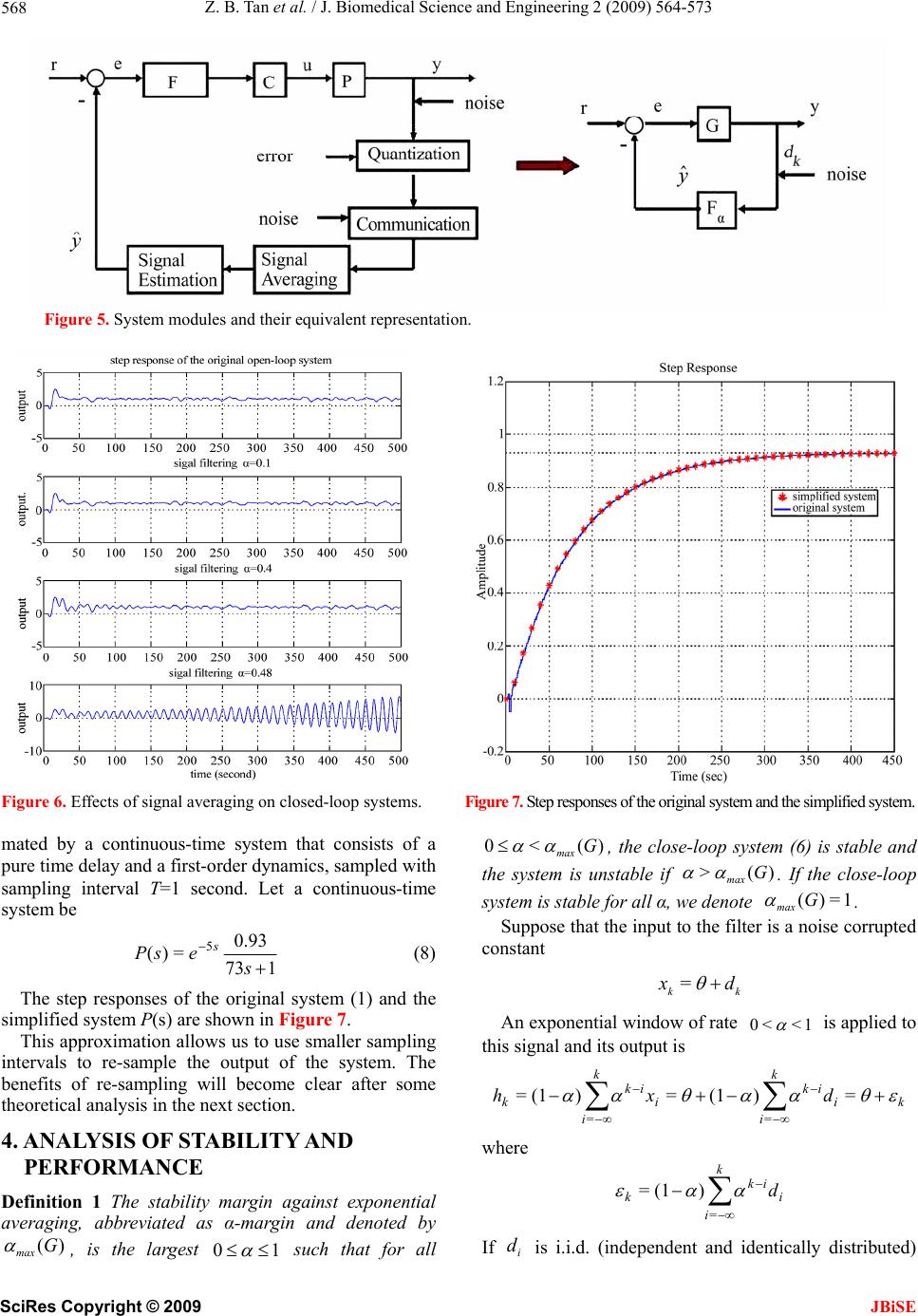

Z. B. Tan et al. / J. Biomedical Science and Engineering 2 (2009) 564-573 568
Figure 5. System modules and their equivalent representation.
Figure 6. Effects of signal averaging on closed-loop systems. Figur e 7. Step responses of the original system and the simplified system.
mated by a continuous-time system that consists of a
pure time delay and a first-order dynamics, sampled with
sampling interval T=1 second. Let a continuous-time
system be
173
0.93
=)( 5


s
esP s (8)
The step responses of the original system (1) and the
simplified system P(s) are shown in Figure 7.
This approximation allows us to use smaller sampling
intervals to re-sample the output of the system. The
benefits of re-sampling will become clear after some
theoretical analysis in the next section.
4. ANALYSIS OF STABILITY AND
PERFORMANCE
Definition 1 The stability margin against exponential
averaging, abbreviated as α-margin and denoted by
)(G
max

, is the largest 10 


such that for all
)(<0 G
max



, the close-loop system (6) is stable and
the system is unstable if . If the close-loop
system is stable for all α, we denote
)(> G
max

1=)(G
max

.
Suppose that the input to the filter is a noise corrupted
constant
=k d
k
x

An exponential window of rate 1<<0

is applied to
this signal and its output is
ki
ik x
 
=i ik d

=
and identically distributed)
k
i
 


)(1
=
i
ik
k
i
d



 
=
)
k
i
k
h  


)(1=
=
If i
d is i.i.d.
where
k
 (1=
(independent
SciRes
Copyright © 2009 JBiSE

Z. B. Tan et al. / J. Biomedical Science and Engineering 2 (2009) 564-573 569
wit 0=
i
Ed and 22 =

i
Ed , then 0=
k
E
h

and
2


2
1
1
= 


k
E
g k
h as a

C, usinn θ can re-
du
onsequently estimate of
ce errors by


 11 We will call .

as the de-
caying rate. Conv (in the mean sqre sense) is
achieved when 1
ergence ua

: 0= lim 2
1k
E 
 .
Consider an entxpr oneial filte
1
1
=)( s sF

onse is
(9)
wh resp ose impulse
0 ,=)(tetf t


1/
p of this
(10)
Now put-output relationshifilter is
Note that
, the in
1=)(
0
dttf



d
d
)(
)(
with sampli
ve


xet
t
1
=)/( 




Wgnals are sampled ng interval
T,
 xtfty t)(=)( 
hen the si
we denote )(= kTxxk and )(=kTyyk. If α is re-
lated to λ and T
 /, we ha by
 =T e
1=
)(1
lim
0
 

T
T
, is approxima ted by For small T)(ty
i
ik
k
i
i
ik x (1
analysis, we ma
ponentia
k
i
i
ikT
k
i
t
k
x
T
xe
T
ey










 



==
/
=
(
))(1
)(1
=)(
In other words, for systemy approxi-
m
Exl
The between
t
dxkTy  
 )/ )(
1
)(
ate the discrete-time filter in (3) by its continuous-time
counterpart in (9). These relationships between discrete-
time averaging and continuous time averaging will be
used to derive stability margins.
4.1. Stability Margin against
Averaging
relationship

and

will allow us to
in
ty margin in the
co
focus on stability analysis continuous time systems
and then transform the results to the discrete-time filters.
This is stated in the following theorem.
Theorem 1 If the exponential stabili
ntinuous-time domain is max

, then
max
max
T
T


=
ln
lim
0 
Proof: This follows from the relationship
We now concentrate on calculation of .
nst nential
av


/
=T e
max

Definition 2 The stability margin agai expo
eraging for the continuous-time closed-loop system,
abbreviated as continuous exponential A-margin and
denoted by )(G
max

, is the smallest 0>

under which
the closed-loop system becomes able. If the
closed-loop system remains stable for all 0>
unst

, we de-
note

=)(G
max

.
Supp =N ose )()/(sDs
ial functions of s
)(sG where
ar
)(sn and )(sd
)(sN
e polynom and coprihat is,
and )(sD do not have common zeros). Then max
me (t

is
the t 0> larges

before the closed-loop systee-
comes unstablonsider the characteristic equation of
the closed-loop system
m b
e. C
0=
)(
)(
1
1
1=)()(1 sD
sN
s
sGsF  


or
0=)()()( sNsDssD 


(11)
which leads to
0=
)()(
)(
1sNsD
ssD

  (12)
This expression leads to the following conclusion.
Theorem 2 The exponential A-margin )(G
max

of
)(sG is the gain margin of
)()(
)(
=)( sNsD
ssD
sH  (13)
We make several interesting observations from (12).
First, from (11), max

may be calculated by using the
Routh-Hurwitz test. Second, (12) is in a standard form
for using root locus technique. So, we may plot the root
locus of the system (13) (it is an improper system) and
detect the

value that reaches marginal stability,
which will b max e

. The root locus plot starts at the
poles of system (13) which are precisely the poles of the
closed-loop system without the averaging filter. Since
SciRes
Copyright © 2009 JBiSE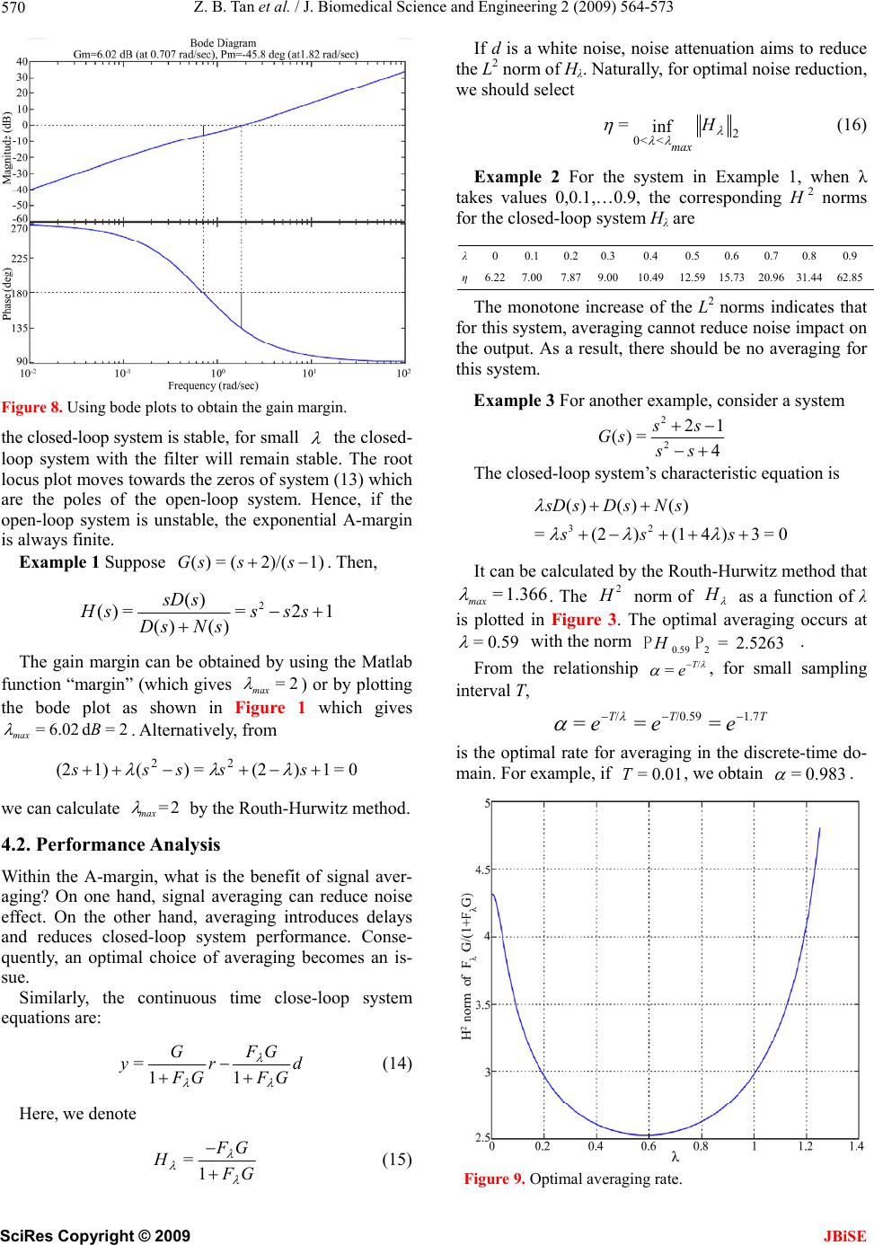

Z. B. Tan et al. / J. Biomedical Science and Engineering 2 (2009) 564-573 570
Figure 8. Using bode plots to obtain the gain margin.
the closed-loop system is stable, for small

the closed-
ppose . Then,
loop system with the filter will remain stable. The root
locus plot moves towards the zeros of system (13) which
are the poles of the open-loop system. Hence, if the
open-loop system is unstable, the exponential A-margin
is always finite.
Example 1 Su1)2)/((=)(  sssG
12=
)()(
)(
=)( 2
sss sNsD
ssD
sH
The gain margin can be obtained by using the Matlab
function “margin” (which gives 2=
max

) or by plotting
the bode plot as shown in Fi which gives
2=d 6.02=B
max
gure 1

. Alternatively, from
0=1)(2=)(1)(2 22  sssss 
we can calculate 2=
max

by the Routh-Hurwitz method.
Analysis
e benefit of signal aver-
ilarly, the continuous time close-loop system
eq
4.2. Performance
Within the A-margin, what is th
aging? On one hand, signal averaging can reduce noise
effect. On the other hand, averaging introduces delays
and reduces closed-loop system performance. Conse-
quently, an optimal choice of averaging becomes an is-
sue.
Sim
uations are:
d
GF
GF
r
GF
G
y





11
= (14)
Here, we denote
(15)
If d is a white noise, noise attenuation aim
the L2 norm of Hλ. Naturally, for op
we should select
s to reduce
timal noise reduction,
GF
GF
H





1
=
2
<<0
inf
=


 H
max
(16)
Example 2 For the system in Exa
takes values 0,0.1,…0.9, the correspo
for the closed-loop system Hλ are
The monotone increase of the L2 norms indicates that
fsmegnneduce n iac
tus ts
th
mple 1, when λ
nding H 2 norms
or this yste, avragin caot roisempt on
he outpt. A a result,here hould be no averaging for
is system.
Example 3 For another example, consider a system
221
2
()
=4
s
s
Gs
ss
The closed-loop system’s characteristic equation is
32
=(2)(14)3=0ss s
() () ()sD sD sNs

 


 
It can be calculated by the Routh-Hurwitz method that
. The
1.366=
max

2
H
norm of as a fution of λ
Figur he optiml averaging occurs at

H
a
nc
is plotted in e 3. T
0.59=

with the norm 2.5263=
0.59 PP H.
ip


/
=T eor small sampling
interval T,
T/ 
2
From the relationsh f
l rate for averaging in the discrete-time do-
main. For example, if , we obtain
,
TT
e1.7/0.59 ee === 
is the optima
0.01=T0.983=

.
λ 0 0.1 0.2 0.3 0.4 0.5 0.6 0.7 0.8 0.9
η6.227.00 7.87 9.0010.49 12.59 15.73 20.9631.4462.85
Figure 9. Optimal averaging rate.
SciRes
Copyright © 2009 JBiSE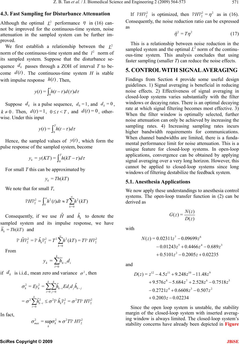

Z. B. Tan et al. / J. Biomedical Science and Engineering 2 (2009) 564-573 571
4.3. Fast Sampling for Disturbance Attenuation
Although the optimal 2
L
performance

in (16) can-
not be improved for the continuous-time system, noise
attenuation in the sampled system can be further im-
proved.
We first establish a relationship between the 2
L
of
-
to be-
norm of the continuous-time system and the norm
its sampled system. Suppose that the disbance se
quence passes through a ZOH of inT
come . The continuous-time system is stable
with imesponse . Then,
2
l
tur
terval
H
k
d
)(td
pulse r)(th
0
()=()()
t
ythtd d

 

Suppose is a pulse sequence, , and
. Th, a
w
k
d
en, d
1=
0
d
nd (td
0=
k
d,
, other-
0Tt <0
ise. Under this input
k1=)(t, 0=)
0
()= ()
T
ytht d

 

Hence, the sampled values of )(ty , which form the
pulse response of the sampled system, become
0
=( )=()
T
k
yyKThkT d

 

For small T this can be approximated by
=()
k
yThkT
We note that for smal l T,
)
22 2
20=0
=() (
k
H
htdt ThT



PP k
Consequently, if we use
H
 and to dene
led systese respe have
)(=
k
h

o
ote th
sampm and its imlnse, wpu
~
kTThhk and
2222
22
=0
== ()=
k
k
2
2
H
hThkTTH


 
PP PPPP
From
k
dhy ~ =iik
i
k
0=
if is i.i.d., mean zero and variance n
2
H
In fact,
2
k
d 2

, the
22
kk
=0 =0
2 2
22
=0
==
=
kk kiijkj
ij
k
i
EyhEd dh
T




P PP
22 2
=
k
ki
hh 


P
222
2
=sup
max k
k
TH  PP
If 2
2
H
PP
is optimized, then 22
2
H=

PP as in (16).
Consequently, the noise reduction ratio can be expressed
as
22
=T

 (17)
This is a relationship between noise reduction in the
sastem and the optimal L2 norm of the continu-
ous-time system. This analysis concludes that using
faster sampling (smaller T) can reduce the noise effects.
V ING
Findings from Section 4 provide some useful design
guidelines. 1) Signal averaging is beneficial in reducing
noise effects. 2) Effectiveness of signal averaging in
closed-loop systems varies substantially with the filter
windows or decaying rates. There is an optimal decaying
rate at which signal filtering becomes most effective. 3)
filter window is optimally selected, further
noise attenuation can only be achieved byng the
sampling rates. 4) Increasing sampling rates incurs
hi ban for com
performance limit for noise attenuation. This is a
unique feature for closed-loop
applications, convergence can be
si
mpled sy
5. CONTROL WITH SIGNAL AERAG
When the
increasi
gherdwidth requirementsmunications.
When channel bandwidths are limited, there is a funda-
mental
systems. In open-loop
obtained by applying
gnal averaging over a very long horizon. However, this
cannot be applied to closed-loop systems since long
windows of filtering destabilize the feedback system.
5.1. Anesthesia Applications
We now apply these understandings to anesthesia control
systems. The open-loop transfer function in (2) can be
derived as
()
()= ()
Nz
Gz Dz
with
76
543
2
() =0.023110.09699
0.012430.4466 0.689
0.51010.2005 0.02235
Nz zz
zzz
zz



and
12 11109
876 5
432
() =4.59.24811.48
9.576 5.6842.528 0.7518
0.2721 0.6608 0.507
Dz zzzz
zzz z
zzz
 


0.2003 0.02234z
Since the open loop system is unstable, the stability
margin of the closed-loop system with inserted averag-
ing window is always limited. The closed-loop system’s
stability concerns have already been depicted in Figure
SciRes
Copyright © 2009 JBiSE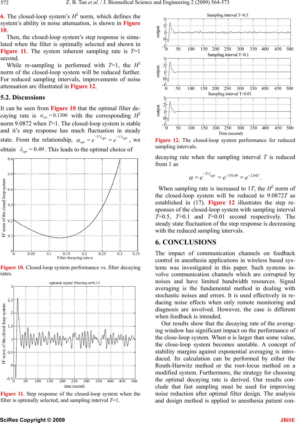

Z. B. Tan et al. / J. Biomedical Science and Engineering 2 (2009) 564-573 572
6. The closed-loop system’s H2 no, which defines the
system’s ability in noise attenuation, is shown in Figure
10.
, the closed-loop system’s step response is simu-
lated when the filter is optimally selected and shown in
Figure 11. The system inherent sampling rate is T=1
second.
While re-sampling is performed with T=1, the H2
norm of the closed-loop system will be reduced further.
uced sampling intervals, improvements of noise
tion are illustrated in Figure 12.
5.2. Discussions
It can be seen from Figure 10 that the optimal filter de-
caying rate is with the corresponding H2
norm 9.0872 wh closed-loop system is stable
and it’
rm
Then
For red
attenua
0.1300=
opt

en T=1. The
s step response has much fluctuation in steady
state. From the relationship, optopt
T
opt ee


1//==  , we
obtain 0.49=
opt

. This leads to the optimal choice of
Figure 10. Closed-loop system performance vs. filter decaying
rates.
Figure 12. The closed-loop system performance for reduced
sampling intervals.
decaying rate when the sampling interval T is reduced
from 1 as
When sampling rate is increased to 1T, the H2 norm of
the closed-loop system will be reduced to 9.0872T as
established in (17). Figure 12 illustrates the step re-
sponses of the closed-loop system with sampling interval
T=0.5, T=0.1 and T=0.01 second respectively. The
steady state fluctuation of the step response is decreasing
with the reduced sampling intervals.
6. CONCLUSIONS
ed sys-
tems was investigated in this paper. Such systems in-
volve communication channels which are corrupted by
noises and have limited bandwidth resources. Signal
averaging is the fundamental method in dealing with
stochastic noises and errors. It is used effectively in re-
ducing noise effects when only remote monitoring and
diagnosis are involved. However, the case is different
when feedback is intended.
Our results show that the decaying rate of the averag-
ing window has significant impact on the performance of
the close-loop system. When α is larger than some value,
the close-loop system becomes unstable. A concept of
stability margins against exponential averaging is intro-
duced. Its calculation can be performed by either the
Routh-Hurwitz method or the root-locus method on a
modified system. Furthermore, the strategy for choosing
the optimal decaying rate is derived. Our results con-
and design method is applied to anesthesia patient con-
.=== 2.04/0.49
/TT
opt
Teee  

The impact of communication channels on feedback
control in anesthesia applications in wireless bas
clude that fast sampling must be used for improving
noise reduction after optimal filter design. The analysis
Figure 11. Step response of the closed-loop system when the
filter is optimally selected, and sampling interval T=1.
SciRes
Copyright © 2009 JBiSE

Z. B. Tan et al. / J. Biomedical Science and Engineering 2 (2009) 564-573
SciRes Copyright © 2009
573
sis is conducted on the basis of the linear
systems. Actually, anesthesia patient models contain non-
linearity. Our future work will consider analysis of non-
l
anean Conference on
Athens-Greece.
erosa, M., and Morari, M.,
trol problems.
Our analy
[6] Talbot, S. L. and Boroujeny, B. F., (2008) Spectral
of the
method of blind carrier tracking for OFDM, IEEE Trans-
actions on Signal Processing, 56(7).
[7] Bataillou, E., Thierry, E., Rix, H., and Meste, O., (1995)
Weighted averaging using adaptive estimation
inear systems.
REFERENCES
[1] Nunes, C. S., Mendonca, T., Lemos, J. M., and Amorim,
P., (2007) Predictive adaptive control of the bispectral
index of the EEG (BIS): Exploring electromyography as
an accessible disturbance, Mediterr
weights, Signal Processing, 44, 5l−66.
[8] Eisenach, J. C., (1999) Reports of Scientific Meetings—
Workshop on Safe Feedback Control of Anesthetic Drug
Delivery, Anesthesilogy, 91, 600–601.
[9] Linkens, D. A., (1992) Adaptive and intelligent control in
anesthesia, IEEE Control Systems Magazine, 6–11.
[10] Wang, L. Y. and Wang, H., (2002) Control-oriented mod-
eling of BIS-based patient response to anesthesia infu-
sion, Internat. Conf. Math. Eng. Techniques in Medicine
Control and Automation,
[2] Gentilini, A., Rossoni-Get al, and Bio. Sci., Las Vegas.
[11] Wang, L. Y. and Wang, H., (2002) Feedback and predic-
tive control of anesthesia infusion using control-oriented
patient models, Internat. Conf. Math. Eng. Techniques in
Medicine and Bio. Sci., Las Vegas.
(2001) Modeling and closed-loop control of hypnosis by
means of bispectral index (BIS) with isoflurane, IEEE
Trans. on Biomedical Engineering, 48, 874−889,.
[3] Dong, C., Kehoe, J., Henry, J., Ifeachor, E. C., Reeve, C.
D., and Sneyd, J. R., (1999) Closed-loop computer con-
trolled sedation with propofol, Proc. of the Anaesthetic
Research Society, 631.
[4] Zhang, X. S., Roy, R. J., and Huang, J. W., (1998) Closed-
loop system for total intravenous anesthesia by simulta-
neously administering two anesthetic drugs, Proc. of the
20th Annual International Conference of the IEEE Engi-
[12] Wang, L. Y., Wang, H., and Yin, G., (2002) Anesthesia
infusion models: Knowledge-based real-time identifica-
tion via stochastic approximation, 41st IEEE Cont. and
Dec. Conf., Las Vegas.
[13] Gan, T. J., et al., (1997) Bispectral index monitoring
allows faster emergence and improved recovery from
propofol, Alfentanil, and Nitrous Oxide Anesthesia, An-
esthesiology, 87, 808–815.
[14] Rosow, C. and Manberg, P. J., (1998) Bispectral index
neering in Medicine and Biology, 3052–3055.
[5] Goldman, J. M., (2006) Medical device connectivity for
improving safety and efficiency, American Society of
Anesthesiologists Newsletters, 70(5),
http://www.asahq.org/Newsletters/2006/05−06/goldman0
5_06.html.
monitoring, Annual of Anesthetic Pharmacology, 2, 1084–
2098.
[15] Ljung, L. and Söderström, T., (1983) Theory and Practice
of Recursive Identification, MIT Press, Cambridge, MA.
JBiSE