 Journal of Mathematical Finance, 2011, 1, 90-97 doi:10.4236/jmf.2011.13012 Published Online November 2011 (http://www.SciRP.org/journal/jmf) Copyright © 2011 SciRes. JMF Stochastic Volatility Jump-Diffusion Model for Option Pricing Nonthiya Makate, Pairote Sattayatham School of Mathematics, Suranaree University of Technology, Nakhon Ratchasima, Thailand E-mail: nonthiyam@hotmail.com, pairote @ s ut . ac.t h Received July 26, 2011; revised September 2, 2011; accepted Septembe r 15, 2011 Abstract An alternative option pricing model is proposed, in which the asset prices follow the jump-diffusion model with square root stochastic volatility. The stochastic volatility follows the jump-diffusion with square root and mean reverting. We find a formulation for the European-style option in terms of characteristic functions of tail probabilities. Keywords: Jump-Diffusion Model, Stochastic Volatility, Characteristic Function, Option Pricing 1. Introduction Let be a probability space with filtration . All processes that we shall consider in this section will be defined in this space. An asset price model with stochastic volatility has been defined by Heston [1] which has the following dynamics: ,,P 0 ttT ddd tt tt S SS tvW , (1) ,dd v ttt vvtv d t W where t is the asset price, S is the rate of return of the asset, t is the volatility of asset returns, v0 is a mean-reverting rate, is the long term variance, 0 is the volatility of volatility, and are standard Brownian motions corresponding to the proc- esses t and t, respectively, with constant correlation S t Wv t W S v . In 1996, Bate [2] introduced the jump-diffusion sto- chastic volatility model by adding log normal jump t to the Heston stochastic volatility model. In the original formulation of Bate, the model has the following form: Y dd d S tttt ttt SStvdW SYN S , (2) dd v ttt vvtvd t W, where is the Poisson process which corresponds to the underlying asset t, t is the jump size of asset price return with log normal distribution and t means that there is a jump the value of the process before the jump is used on the left-hand side of the formula. Moreover, in 2003, Eraker Johannes and Polson [3] extended Bate’s work by incorporating jumps in volatility and their model is given by S t NS YS ddd S tttttt SS tvW SYN d S t , (3) ddd vv ttttv vvtvWZ d t N. Eraker et al. [3] developed a likelihood-based estima- tion strategy and provided estimates of parameters, spot volatility, jump times, and jump sizes using S&P 500 and Nasdaq 100 index returns. Moreover, they examined the volatility structure of the S&P and Nasdaq indices and indicated that models with jumps in volatility are pre- ferred over those without jumps in volatility. But they did not provide a closed-form formula for the price of a European call option. In this paper, we would like to consider the problem of finding a closed-form formula for a European call option where the underlying asset and volatility follow the Model (3). This formula will be useful for option pricing rather than an estimation of it as appeared in Eraker’s work. The rest of the paper is organized as follows. In Sec- tion 2, we briefly discuss the model descriptions for the option pricing. The relationship between stochastic dif- ferential equations and partial differential equations for the jump-diffusion process with jump stochastic volatil- ity is presented in Section 3. Finally, a closed-form for- mula for a European call option in terms of characteristic functions is presented. 2. Model Descriptions It is assumed that a risk-neutral probability measure  91 N. MAKATE ET AL. exists, the asset price t under this measure follows a jump- diffusion process, and the volatility t follows a pure mean reverting and square root diffusion process with jump, i.e. our models are governed by the following dynamics: Sv ddd SS tt d S t ttt SSr mtvSYN t W , (4) dddd vv tt ttt vvtWZN t v, where t, t, , S v , , and are defined as in Bate’s model, is the risk-free interest rate, and are independent Poisson processes with constant in- tensities S t Wv t W rS t N v t NS and v respectively. is the jump size of the asset price return with density t Y Y and :m t and t EY is the jump size of the volatility with density Z. Moreover, we assume that the jump processes and are independent of standard Brownian motions and . z t N S t W X S t Nv v t W 3. Partial Integro-D if f e r en t i al Equations Consider the process where 12 , ttt XX 1 t and 2 t are processes in and satisfy the following equations: 112 12 11 d,,,, ttt tt tt 11 dt 1 d t d ft XXtW XY XXt N XXt g dg (5) 212 12 22 2 d,,,, d ttttt tt X ftXXtW ZN 2 d t where 112 ,, gf and 2 are all continuously differenti- able, and are standard Brownian motions 1 t W 2 d t W with 12 d, Corr Wtt W, and are 1 t N 2 t N independent Poisson processes with constant intensities 1 and 2 respectively. Since every compound Poisson process can be repre- sented as an integral form of a Poisson random measure [4] then the last term on the right hand side of (5) can be written as follows: 11 11 00 dd tt ss snnsQ 1 1 t N n d, YNXYqJ sq X N n 2 2 1 00 dd t tt ssnRd, NZrJs r where n are i.i.d. random variables with density Y Y and Q is a Poisson random measure of the process 1 t 1 tn n with intensity measure , N QY ddqt 1 Yn are i.i.d. random variables with density and ,z Z is a Poisson random measure of the process with 2 1 t N t n R n Z intensity measure . 2dd Zrt Let 12 ,Uxx be a bounded real-valued function and twice continuously differentiable with respect to 1 and 2 and 12 12 121 2 ,,, , TT tt uxxtEUX XXxXx (6) By the two dimensional Dynkin formula [5], is a solution of the partial integro-differential equation (PIDE) u 12 12 (1) 12 12 (2) 12 12 ,, 0,, ,, ,,d ,, ,,d Y Z uxxt uxxt t uxyxtuxxty y uxxztuxxtz z subject to the final condition 12 12 ,, ,uxxT Uxx. The notation is defined by 12 12 12 12 12 22 212 12 112 2 12 1 2 212 22 2 ,, ,, ,, ,, ,, 1 2 ,, 1 2 uxxt uxxt Au xxtff xx uxxt uxxt ggg xx x uxxt gx (7) 4. A Closed-Form Formula for the Price of a European Call Option Let C denote the price at time t of a European style call option on the current price of the underlying asset with strike price and expiration time . t S K T The terminal payoff of a European call option on the underlying stock with strike price is t SK max ,0 T SK. This means that the holder will exercise his right only if and then his gain is T. Otherwise, if T SKSK T SK, then the holder will buy the underlying asset from the market and the value of the option is zero. Assuming the risk-free interest rate is constant over the lifetime of the option, the price of the European call at time t is equal to the discounted conditional expected payoff r Copyright © 2011 SciRes. JMF  N. MAKATE ET AL. 92 () () ,,;, max, 0, ,d ,d 1,d e (,)d 1(,)d [|,] e tt rT tTtt rT tTTttTTtt T KK tTTttT rT tK t rT tTtt T K tTTttT TttK rT t CSvtKT eE SKSv eSPSSvS KPSSvS SSPSSvS S KePSSvS SSPSSvS ESSv K () 12 (,)d (,,;,)(,,;,) Ttt T K rTt ttttt PSSvS SPSvtKTKePSvtKT (8) where is the expectation with respect to the risk- E neutral probability measure, , Ttt SSv is the cor- responding conditional density given and , tt Sv 1,,;,,d, ttTTtt TTtt K PSvtKTSP SSvSESSv Note that 1 is the risk-neutral probability that (since the integrand is nonnegative and the inte- gral over is one), and finally that P T SK 0, 2,,;,, d Pr ob(|,) ttTttT K Tt PSvtKTPSSvS SKSv t is the risk-neutral in-the-money probability. Moreover, ,e rTt Ttt t ESSvS for . 0t Assume that the asset price t and the volatility t satisfy (4), we would like to compute the price of a European call option with strike price S v and maturity . To do this, we make a change of variable from t to , i.e. where satisfies (4) and its inverse T S ln t L tt St S t. Denote the logarithm of the strike price. By the jump-diffusion chain rule, satisfies the SDE SelnkK ln t S lnddln 1d 2 SS t ttt v dSrmt vWYN S tt (9) Applying the two-dimensional Dynkin formula [5] for the price dynamics (9) and volatility t in system (4), we obtain the value of a European-style option, as a function of the stock log-return denoted by v t L ln ,, ,, t t L S tt v ln ,,;,;, ,,; , ;, , k tt t K t CLvtkTCevteT Cevte T CS tKT i.e., ,,;,max T L e,0 , rT ttt ClvtkTeEKL lv v and satisfies the following PIDE: 0,,; ,,;, ,,;,d ,,;, ,,;,d SY vZ CClvtkT t ClyvtkTvtkTy y ClvztkTvtkTzz , Cl Cl (10) Here the operator as in (7) is defined by 22 2 2 2 ,, ;, 1 2 1 2 SCC ClvtkTrmvv lv CC vv lvl C v 2 1 2 C vr In the current state variable, the last line of (8) becomes 12 ,,;, ,,;,,,;, lkrTt ClvtkTeP lvtkTePlvtkT (11) where ,,;,:,,;,,1,2 lk jj PlvtkTPevteT j . The following lemma shows the relationship between and in the option value of (11). 1 P 2 P Lemma 1 The functions and 2 in the option value of (11) satisfy the following PIDEs 1 P P 11 1 1 1 1 0,,;, 1,,:, S Sy Y PP PlvtkT v tl P vrmP v ePlyvtkT y d y and subject to the boundary condition at expiration time tT ; 1,, ;,1 lk PlvTkT (12) moreover, satisfies the equation 2 P 2 22 0,,;, PPlvtkT rP t , Copyright © 2011 SciRes. JMF  93 N. MAKATE ET AL. and subject to the boundary condition at expiration time ; tT 2,,;,1 lk PlvTkT , (13) The operator is defined by 2 2 2 2 2 2 ,,;, 11 :22 1 2 ,,;, ,,;,d ,,;, ,,;,d S SY vZ flvtkT fff rmvvv lv l f f vvrf lv v . lyvtkTflvtkTyy lvztkTf lvTkTzz (14) Note that if and otherwise 101 lk1lk lk . The following lemma shows how to calculate the functions and as they appeared in Lemma 1. 1 P 2 P Lemma 2 The functions and can be calculated by the inverse Fourier transforms of the characteristic function, i.e. 1 P 2 P 0 ,,;, 11 ,,;, Red 2π ixk j j eflvtkT PlvtkT x ix , for with denoting the real component of a complex number. By letting 1, 2jRe[ ] Tt . 1) The characteristic function 1 is given by 11 ,,;, expixlf lvtxtgvh 1 , where 1 1 22 11 1 11 11 2 1e he 1 SS rmixm 1 1 11 11 2 1 1 1 2ln 12 1d 1d ix y SY vZ zh e eyy ezz , 11ix and 22 11 1 ix ix. 2) The characteristic function 2 is given by 222 ,,;, exp lvtxtgvhixl r, where 2 2 22 22 22 22 22 1e he , 2ix S rmr 2 2 22 22 2 2 1 2ln 12 1d1 Sixy v YZ zh e eyyez dz 2ix and 22 22 1ix ix . In summary, we have just proved the following main theorem. Theorem 3 The value of a European call option of (4) is 12 ,,;, ,,;,,,;, lkrTt ClvtkTeP lvtkTePlvtkT where and are given in Lemma 2. 1 P 2 P 5. Conclusions This paper has proposed asset price dynamics to accom- modate both jump-diffusion and jump stochastic vola- tility. Under this proposed model, an analytical solution is derived for a European call option via the characteris- tic function. 6. Acknowledgements This research is (partially) supported by The Centre of Excellence in Mathematics, the Commission on Higher Education (CHE). Address: 272 Rama VI Road, Ratchathewi District, Bangkok, Thailand. 7. References [1] S. L. Heston, “A Close Form Solution for Options with Stochastic Volatility with Applications to Bond and Cur- rency Options,” The Review of Financial Studies, Vol. 6, No. 2, 1993, pp. 327-343. doi:10.1093/rfs/6.2.327 [2] D. Bates, “Jump and Stochastic Volatility: Exchange Rate Processes Implicit in Deutsche Mark in Options,” Review of Financial Studies, Vol. 9, No. 1, 1996, pp. 69-107. tp://dx.doi.org/10.1093/rfs/9.1.69 Copyright © 2011 SciRes. JMF  N. MAKATE ET AL. Copyright © 2011 SciRes. JMF 94 [3] B. Eraker, M. Johannes and N. Polson, “The Impact of Jumps in Volatility and Returns,” The Journal of Finance, Vol. 58, No. 3, 2003, pp. 1269-1300. doi:10.1111/1540-6261.00566 [4] R. Cont and P. Tankov, “Financial Modeling with Jump Processes,” CRC Press, Boca Raton, 2004. [5] F. B. Hanson, “Applied Stochastic Process and Control for Jump Diffusions: Modeling, Analysis and Computation,” Society for Industrial and Applied Mathematics, Phila- delphia, 2007  95 N. MAKATE ET AL. Appendix Proof of Lemma 1. We plan to substitute (11) into (10). Firstly, we compute 12 2 krTt krTt lPP Cee re ttt P 12 1 krTt ll P CeePe ll l 12 krTt lPP Cee vv v 22 2 11 1 22 2 krTt lll PP CeeePe l ll 2 2 P l 22 2 11 krTt ll PP Ceee lv lv vlv 2 P 22 2 12 22 krTt lPP Cee vv 2 v , 1 1 ,,;, ,,;, ,,;, ,,;, ly krTt Cl yvtkTClvtkT ePlyvtkT ePlyvtkT 12 11 11 11 1 1 ,,;,,,;, ,,;, ,,;, ,,;, ,,;, ,,;,,,;, 1,,;, ,,;, krTt l ly ll krTt ly l eP lvtkTePlvtkT eeP lyvtkTPlyvtkT eP lyvtkTeP lvtkT eP lyvtkTP lvtkT eePl yvtkT eP lyvtkT 1 21 ,,;, ,,;,,,;, krTt PlvtkT ePlyvtkTP lvtkT and 12 12 11 22 , ,;,,,;, , ,;,, ,;, ,,;, ,,;, , ,;,,,;, , ,;,,,;, krTt l krTt l l krTt ClvztkTClvtkT ePlvztkTePlvztkT eP lvtkTePlvtkT eP lvztkTP lvtkT eP lvztkTPlvtkT We substitute all terms above into (10) and separate it by assumed independent terms of and . This gives two PIDEs for the risk-neutralized probability for : (Equation (15)) 1 P2 P (, ,;,),1,2 j PlvtkT j 2 11111 11 2 22 2 11 1 11 1 1 2 1 11 0()2 22 11, ,;,, ,; ,(, ,;,)d 2 , S Sy Y v PPPPP rmv PvvP tlvl l PP P vvrPePlyvtkTPlyvtkTPlvtkT lv vv Plv 1 ,; ,,,; ,d Z ztkTPlvtkTzz yy (15) subject to the boundary condition at the expiration time according to (12). tT By using the notation in (14), PIDE (15) becomes 11 1 1 1 1 1 1 0,,;, 1,,;, :,,;, S Sy Y PP PlvtkTv tl P vrmP v ePlyvtkT y PPlvtkT t d y For 2,,;,PlvtkT: 22 2 1 02 S PP rP rm vv tl 22 2 2 22 2 2 22 22 22 11 22 ,,;, ,,;,d , ,;,,,;,d SY vZ PP P vv vrP lv lv P lyvtkTP lvtkTyy PlvztkTPlvtkTzz (16) subject to the boundary condition at the expiration time tT according to (13). Again, by using the notation in (14), PIDE (16) becomes 2 22 0[](,,;,) PPlvtkT rP t 2 P v 2 22 :[](,,; PPlvtkT t,). Copyright © 2011 SciRes. JMF  N. MAKATE ET AL. 96 The proof of Lemma 1 is now completed. For the characteristic functions for 1, 2j ,,;, j PlvtkT, with respect to the variable are defined by k ,,;, :d,,;, ixk jj lvtxTeP lvtkT , with a minus sign to account for the negativity of the measure d P. Note that also satisfies similar PIDEs ,,;, 0 jjj fflvtxT t , (17) with the respective boundary conditions ,,;,d ,,;, d ixk jj ixk ixl lvtxTePlvtkT ekl e k since d,,;,d1 dd jlk PlvTkTHl kklk . Proof of Lemma 2 1) To solve for the characteristic function explicitly, letting Tt be the time-to-go, we conjecture that the function 1 is given by 11 ,,;, exp 1 lvtxtgvhixl (18) and the boundary condition 11 00 0gh . This conjecture exploits the linearity of the coefficient in PIDE (17). Note that the characteristic function 1 always exists. In order to substitute (18) into (17), firstly we com- pute 1 111 f vh f t 1 1 fixf l 1 1 fh v 1 f 2 2 1 1 2 f f l 2 1 1 fixh f lv 1 2 2 1 11 2 fhf v 1 1 1,,;, ,,;, 1,,;, ixy f lyvtxtflvtxt eflvtxt 1 11 1 , ,;,,,;, 1,,;, zh f lvztxtflvtxt eflvtxt and 11 1 1 1,,;, 1 1,,;, yy yixy gvhixly eflyvtxt ee eeflvtxt Substituting all the above terms into (17) and after canceling the common factor of 1 , we get a simplified form as follows: 1 11 2 1 22 11 1 1 02 1 2 1 2 1d 1d. S S SY vZ y zh ix vhrmv ix vvh vx vixhvhm eyy ezz By separating the order and ordering the remaining terms, we can reduce it to two ordinary differential equa- tion (ODEs), v 22 2 111 11 1 22 hh ixhix 1 2 x (19) and 1 11 11d 1d. SS SY vZ y zh ix hrmix ey ez m y z (20) Let 11ix and substitute it into (19). We get 22 1 111 22 22 11 12 22 11 12 211 11 11 22 2 11 1 2 244 1 12 22 2441 2 1 2 hhhixix ix ix h ix ix h hh where 22 11 1ix ix . By the method of variable separation, we have 2 1 11 11 11 22 2d d h hh . Copyright © 2011 SciRes. JMF 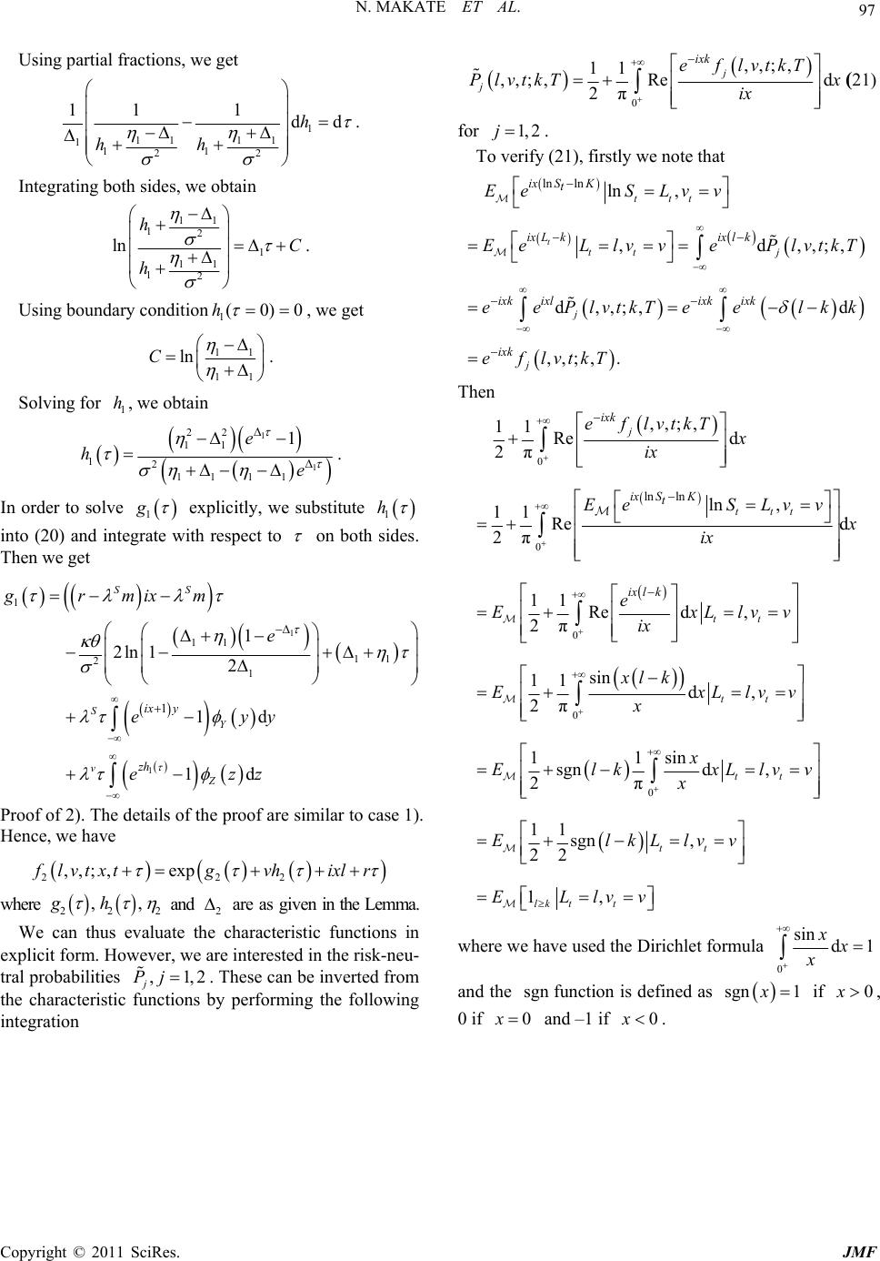 N. MAKATE ET AL. Copyright © 2011 SciRes. JMF 97 Using partial fractions, we get 1 11 11 111 22 11 1 dd h hh . 0 ,,;, 11 ,,;, Red 2π j j ixk eflvtkT PlvtkT x ix (21) for 1,2j . To verify (21), firstly we note that ln lnln , ,d, d,,;, d ,,;, . t ttt ttj j j ix SK t ix ix Lk ixk ixlixk ixk ixk lk Ee SLvv EeLlvv ePlvtkT eePlvtkTee lkk eflvtkT Integrating both sides, we obtain 11 12 1 11 12 ln hC h . ,;, Using boundary condition1(0)0h , we get 11 11 lnC . Then Solving for , we obtain 1 h 1 1 22 11 12 11 11 1e he . In order to solve 1 g explicitly, we substitute 1 h into (20) and integrate with respect to on both sides. Then we get 1 1 1 11 11 2 1 1 1 2ln12 1d 1d SS SY vZ y zh ix grmixm e eyy ezz Proof of 2). The details of the proof are similar to case 1). Hence, we have 0 0 0 0 ln ln ,,;, 11Re d 2π ln , 11Re d 2π 11Red , 2π sin 11 d, 2π 11 sgn 2π j ttt tt tt ixk ix SK t ix lk eflvtkTx ix Ee SLvv ix e ExLlv ix xl k ExLlv x Elk 222 ,,;, exp lvtxtgvhixl r v v 0 sin d, 11 sgn , 22 1, tt tt lk tt xxLlvv x ElkLlvv ELlvv 2 where 22 ,,gh and are as given in the Lemma. 2 We can thus evaluate the characteristic functions in explicit form. However, we are interested in the risk-neu- tral probabilities . These can be inverted from the characteristic functions by performing the following integration ,1,2 j Pj where we have used the Dirichlet formula 0 sin d1 xx x and the function is defined as if , 0 if sgn 0 sgn 1x0x x and –1 if 0 x.
|