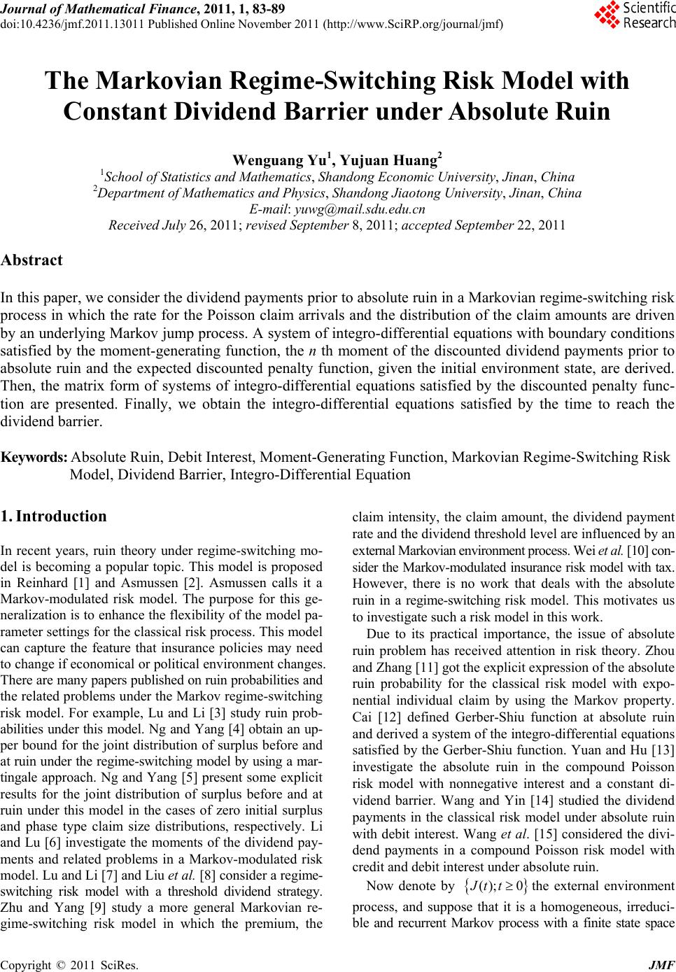
 Journal of Mathematical Finance, 2011, 1, 83-89 doi:10.4236/jmf.2011.13011 Published Online November 2011 (http://www.SciRP.org/journal/jmf) Copyright © 2011 SciRes. JMF The Markovian Regime-Switching Risk Model with Constant Dividend Barrier under Absolute Ruin Wenguang Yu1, Yujuan Huang2 1School of Statistics and Mathematics, Shandong Economic University, Jinan, China 2Departme n t of Mathematics and Physics, Shandong Jiaotong University, Jinan, China E-mail: yuwg@mail.sdu.edu.cn Received July 26, 2011; revised September 8, 2011; accepted September 22, 2011 Abstract In this paper, we consider the dividend payments prior to absolute ruin in a Markovian regime-switching risk process in which the rate for the Poisson claim arrivals and the distribution of the claim amounts are driven by an underlying Markov jump process. A system of integro-differential equations with boundary conditions satisfied by the moment-generating function, the n th moment of the discounted dividend payments prior to absolute ruin and the expected discounted penalty function, given the initial environment state, are derived. Then, the matrix form of systems of integro-differential equations satisfied by the discounted penalty func- tion are presented. Finally, we obtain the integro-differential equations satisfied by the time to reach the dividend barrier. Keywords: Absolute Ruin, Debit Interest, Moment-Generating Function, Markovian Regime-Switching Risk Model, Dividend Barrier, Integro-Differential Equation 1. Introduction In recent years, ruin theory under regime-switching mo- del is becoming a popular topic. This model is proposed in Reinhard [1] and Asmussen [2]. Asmussen calls it a Markov-modulated risk model. The purpose for this ge- neralization is to enhan ce the flexibility of the model pa- rameter settings for the classical risk process. This model can capture the feature that insurance policies may need to change if economical or political env ironment chan ges. There are many papers published on ruin probabilities and the related problems under the Markov regime-switching risk model. For example, Lu and Li [3] study ruin prob- abilities under this model. Ng and Yang [4] obtain an up- per bound for the joint distribution of surplus before and at ruin under the regime-switching model by using a mar- tingale approach. Ng and Yang [5] present some explicit results for the joint distribution of surplus before and at ruin under this model in the cases of zero initial surplus and phase type claim size distributions, respectively. Li and Lu [6] investigate the moments of the dividend pay- ments and related problems in a Markov-modulated risk model. Lu and Li [7] and Liu et al. [8] consider a regime- switching risk model with a threshold dividend strategy. Zhu and Yang [9] study a more general Markovian re- gime-switching risk model in which the premium, the claim intensity, the claim amount, the dividend payment rate and the dividend threshold level are influenced by an external Markovi an environm ent process. Wei et al. [10] con- sider the Markov-modulated insurance risk model with tax. However, there is no work that deals with the absolute ruin in a regime-switching risk model. This motivates us to investigate such a risk model in th is work. Due to its practical importance, the issue of absolute ruin problem has received attention in risk theory. Zhou and Zhang [11] got the explicit expression of the absolu te ruin probability for the classical risk model with expo- nential individual claim by using the Markov property. Cai [12] defined Gerber-Shiu function at absolute ruin and derived a system of the integro-differential equations satisfied by the Gerber-Shiu function. Yuan and Hu [13] investigate the absolute ruin in the compound Poisson risk model with nonnegative interest and a constant di- vidend barrier. Wang and Yin [14] studied the dividend payments in the classical risk model under absolute ruin with debit interest. Wang et al. [15] considered the divi- dend payments in a compound Poisson risk model with credit and debit interest under absolute ruin. Now denote by (); 0Jt tthe external environment process, and suppose that it is a homogeneous, irreduci- ble and recurrent Markov process with a finite state space 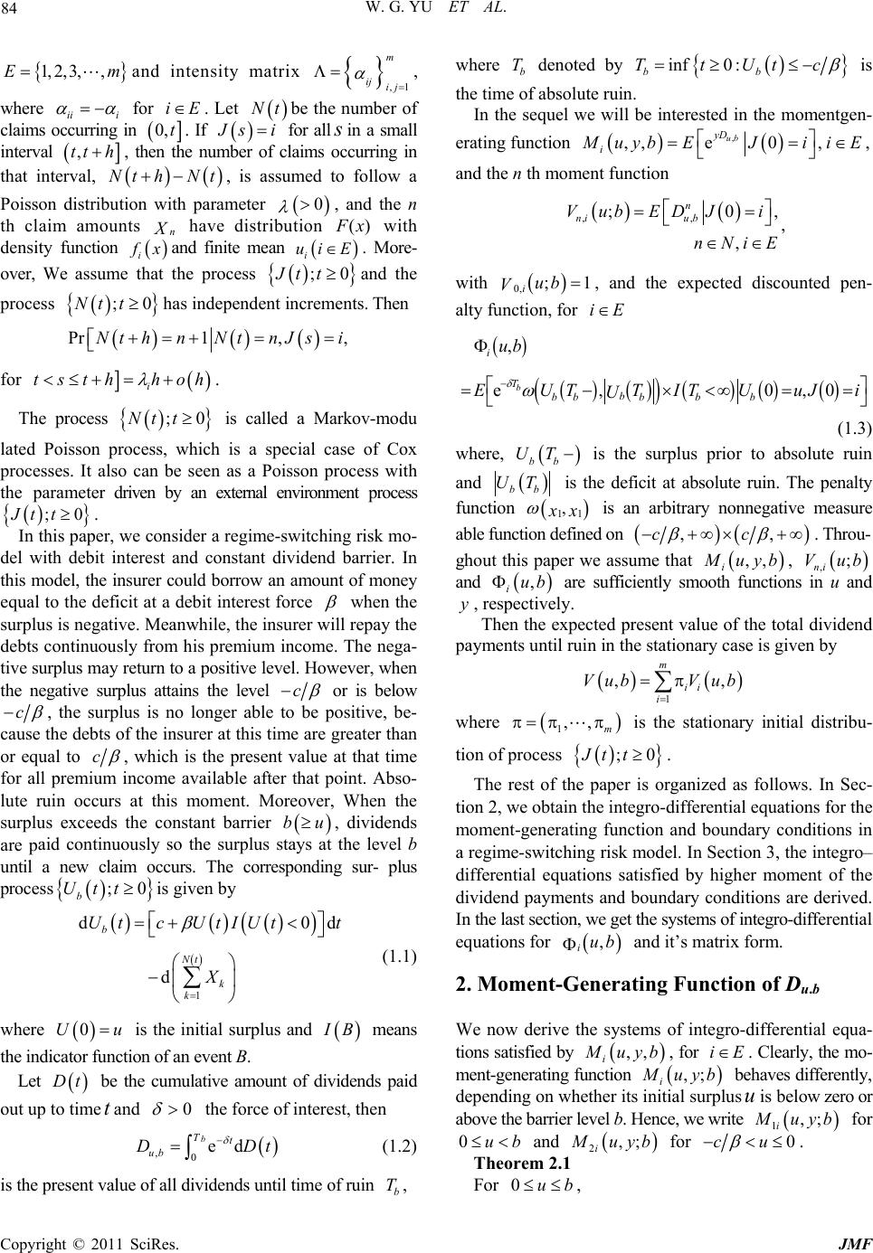 W. G. YU ET AL. 84 1,2,3,,Em and intensity matrix ,1 m ij ij , where iii for i. Let be the number of claims occurring in E Nt 0,t. If si for allin a small interval s ,tt h Nt , then the number of claims occurring in that interval, , is assumed to follow a h N t Poisson distribution with parameter , and the n th claim amounts n 0 i have distribution () i x with density function i xand finite mean i uiE . More- over, We assume that the process and the ;0Jt t process has independent increments. Then ;0Nt t Pr1, , Nt hnNtnJsi for i tsth hoh . The process is called a Markov-modu ;0Nt t lated Poisson process, which is a special case of Cox processes. It also can be seen as a Poisson process with the parameter driven by an external environment process ;0Jt t. In this paper, we consider a regime-switching risk mo- del with debit interest and constant dividend barrier. In this model, the insurer could borrow an amount of money equal to the deficit at a debit interest force when the surplus is negative. Meanwh ile, the insurer will repay the debts con tinuously from his premium income. The nega- tive su rplus may return to a p osit ive leve l. Ho wev er, when the negative surplus attains the level c or is below c , the surplus is no longer able to be positive, be- cause the deb ts of the insurer at this time are greater than or equal to c , which is the present value at that time for all premium income available after that point. Abso- lute ruin occurs at this moment. Moreover, When the surplus exceeds the constant barrier , dividends are paid continuously so the surplus stays at the level b until a new claim occurs. The corresponding sur- plus process is given by b u ;0 b Utt 1 d d b Nt k k Utc UtIUtt X 0d u (1.1) where is the initial surplus and 0U B means the indicator function of an event B. Let be the cumulative amount of dividends paid out up to timetand Dt 0 the force of interest, then ,0ed b Tt ub D Dt (1.2) is the present value of all dividends until time of ruin , b T where denoted by b T inf 0: bb TtUtc is the time of absolute ruin. In the sequel we will be interested in the momentgen- erating function , ,,e0, ub yD i uybEJi i E , and the n th moment func tion ,, ;0 , n ni ub Vub EDJi nNiE , , with 0, ; iub V1 , and the expected discounted pen- alty function, for iE , e, 0, b i Tb bbbb b ub EUTTITUuJ U 0i (1.3) where, bb UT is the surplus prior to absolute ruin and bb UT is the deficit at absolute ruin. The penalty function 11 , x is an arbitrary nonnegative measure able function defined on ,,cc . Throu- ghout this paper we assume that ,, i uyb, ,; ni Vub and , iub are sufficiently smooth functions in u and , respectively. yThen the expected present value of the total dividend payments until ruin in the stationary case is given by 1 ,, m ii i VubVub where 1,, m is the stationary initial distribu- tion of process ;0tJt . The rest of the paper is organized as follows. In Sec- tion 2, we obtain the integro-differential equations for the moment-generating function and boundary conditions in a regime-switching risk model. In Section 3, the integro– differential equations satisfied by higher moment of the dividend payments and boundary conditions are derived. In the last section, we get the systems of integro-differential equations for , iub and it’s matrix form. 2. Moment-Generating Function of Du.b We now derive the systems of integro-differential equa- tions satisfied by ,, i uyb i , for . Clearly, the mo- ment-generating function iE ,; uyb behaves differently, depending on whether its initial surplusuis below zero or above the barrier level b. He nce, we write 1,; i uyb for 0ub and 2,; i uyb for 0uc . Theorem 2.1 For 0ub , Copyright © 2011 SciRes. JMF 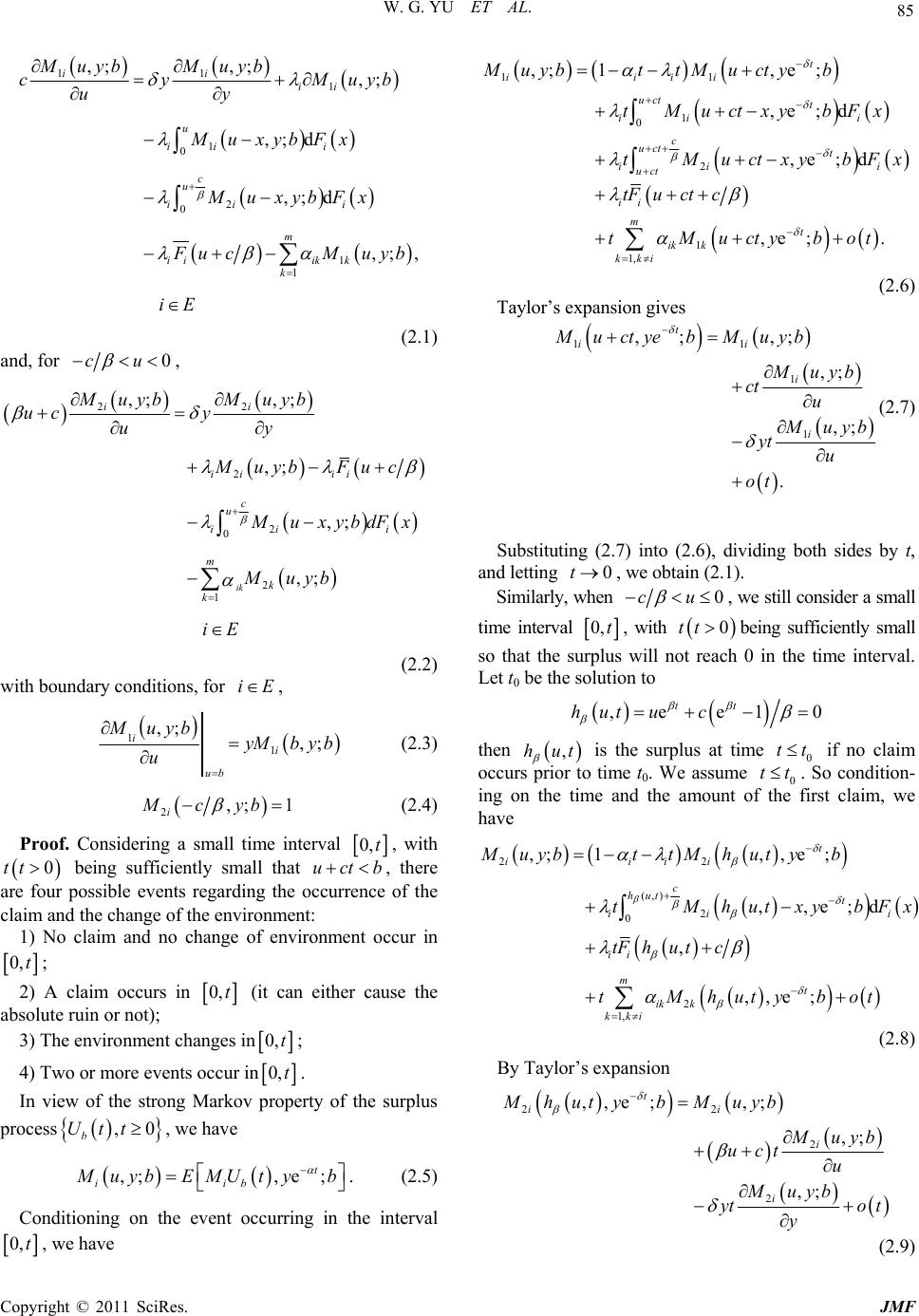 85 W. G. YU ET AL. 11 1 1 0 2 0 1 1 ,;,; ,; ,; d ,; d ,; , ii ii u ii i c u ii i m iiik k k M uybM uyb cy Mu uy MuxybFx MuxybFx yb ucM uyb iE (2.1) and, for 0cu , 22 2 2 0 2 1 ,; ,; ,; ,; ,; ik ii ii ii c u ii i m k k Muyb Muyb uc y uy Muyb Fuc uxybdFx Muyb iE (2.2) with boundary conditions, for , iE 11 ,; ,; ii ub Muyb yMby b u (2.3) 2,; 1 i Mcyb (2.4) Proof. Considering a small time interval 0,t tb , with being sufficiently small that , there are four possible events regarding the occurrence of the claim and the change of the environment: 0tt uc 1) No claim and no change of environment occur in 0,t; 2) A claim occurs in 0,t (it can either cause the absolute ruin or not); 3) The environment changes in 0,t; 4) Two or more events occur in 0,t. In view of the strong Markov property of the surplus process , we have ,0 b Utt ,;,e; t iib uybEMUt yb . (2.5) Conditioning on the event occurring in the interval 0,t, we have 11 1 0 2 1 1, ,;1,e ; ,e; d ,e; d ,e ;. t iiii uct t ii i c uct t ii uct ii mt ik k kki Muybt tMuctyb tMuctxybFx tMuctxybF tF uctc tMuctybot i x (2.6) Taylor’s expansion gives 11 1 1 ,; ,; ,; ,; . t ii i i Muctb Muyb ye uyb ct u uyb yt u ot (2.7) Substituting (2.7) into (2.6), dividing both sides by t, and letting , we obtain (2.1). 0t Similarly, when 0cu , we still consider a small time interval 0,t, with 0ttbeing sufficiently small so that the surplus will not reach 0 in the time interval. Let t0 be the solution to ,e e1 tt hut uc 0 then ,hut is the surplus at time 0 if no claim occurs prior to time t0. We assume 0. So condition- ing on the time and the amount of the first claim, we have tt tt 22 (,) 2 0 2 1, ,;1, ,e; ,,e;d , ,,e; t iiii c hut t ii ii mt ik k kki MuybttMhutyb tMhutxybF tFhutc tMhutybot i x (2.8) By Taylor’s expansion 22 2 2 ,,e; ,; ,; ,; t ii i i Mhutyb Muyb uyb uctu Muyb yto t y (2.9) Copyright © 2011 SciRes. JMF 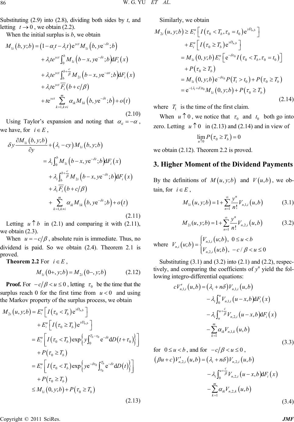 W. G. YU ET AL. 86 Substituting (2.9) into (2.8), dividing both sides by t, and letting , we obtain (2.2) . 0t When the initial surplus is b, we obtain 11 1 0 2 1 1, ,;1e,e; ,e; d ,e;d e e,e; yct t iiii b yct t iii c b yct t ii b yct ii m yct t ik k kki Mbybt tMbyb teMbx ybFx teMbxybFx tFbc tMbybo i t (2.10) Using Taylor’s expansion and noting that ii , we have, for , iE 11 1 0 2 1 1, ,; ,; ,e; d ,e; d ,e ; iii bt ii i c bt ii i b ii mt ik k kki Mbyb ycyMbyb y Mbxy bFx bxy bFx Fb c byb ot (2.11) Letting in (2.1) and comparing it with (2.11), we obtain (2.3). ub When uc , absolute ruin is immediate. Thus, no dividend is paid. So we obtain (2.4). Theorem 2.1 is proved. Theorem 2.2 For , iE 12 0,; 0,; ii yb Myb (2.12) Proof. For 0cu , letting 0 be the time that the surplus reach 0 for the first time from and using the Markov property of the surplus process, we obtain 0u , , 0 0 0 20 0 00 0 0 0 0 10 ,; e e expe d expee d 0, ; ub i ub i b i b i yD u ib yD ub T ut b b T ut b b ib Muyb EIT EI T EI TyDt PT EI TyDt PT MybP T (2.13) Similarly, we obtain , , 0 0 0 2000 0 10 0 110 ()10 ,;, e e 0, ;e, 0, ;e e0,; ub i ub i i yD u ib yD u ib u ib b ib tib Muyb EITt EI T 00 0 yb EITt PT ybPT tPT MybPT (2.14) where is the time of the first claim. 1 T When 0u , we notice that 0 and both go into zero. Letting 0 t 0u in (2.13) and (2.14) and in view of 0 0 lim 0 b uPT we obtain (2.12). Theorem 2.2 is proved. 3. Higher Moment of the Dividend Payments By the definitions of ,; uyb and , we ob- tain, for ,Vub iE , 1, 1 ,; 1, ! n i n y 1,n i uybV ub n (3.1) 2 1 (,;) 1, ! n i n y ,2,n i uybVub n (3.2) where ,1, , ,2, ;,0 ;;, /0 ni ni ni Vub ub Vub Vub cu Substituting (3.1) and (3.2) into (2.1) and (2.2), respec- tively, and comparing the coefficients of yn yield the fol- lowing integro-differential equations: ,1, ,1, ,1, 0 ,2, ,1, 1 ,, ,d ,d , nii ni u inii c u ini i u m ik n k k cVubnVub VuxbFx VuxbFx Vub (3.3) for 0ub , and for 0cu , ,2, ,2, ,2, 0 ,2, 1 ,, ,d , nii ni c u ini i m ik nk k ucVubnV ub VuxbFx Vub (3.4) Copyright © 2011 SciRes. JMF 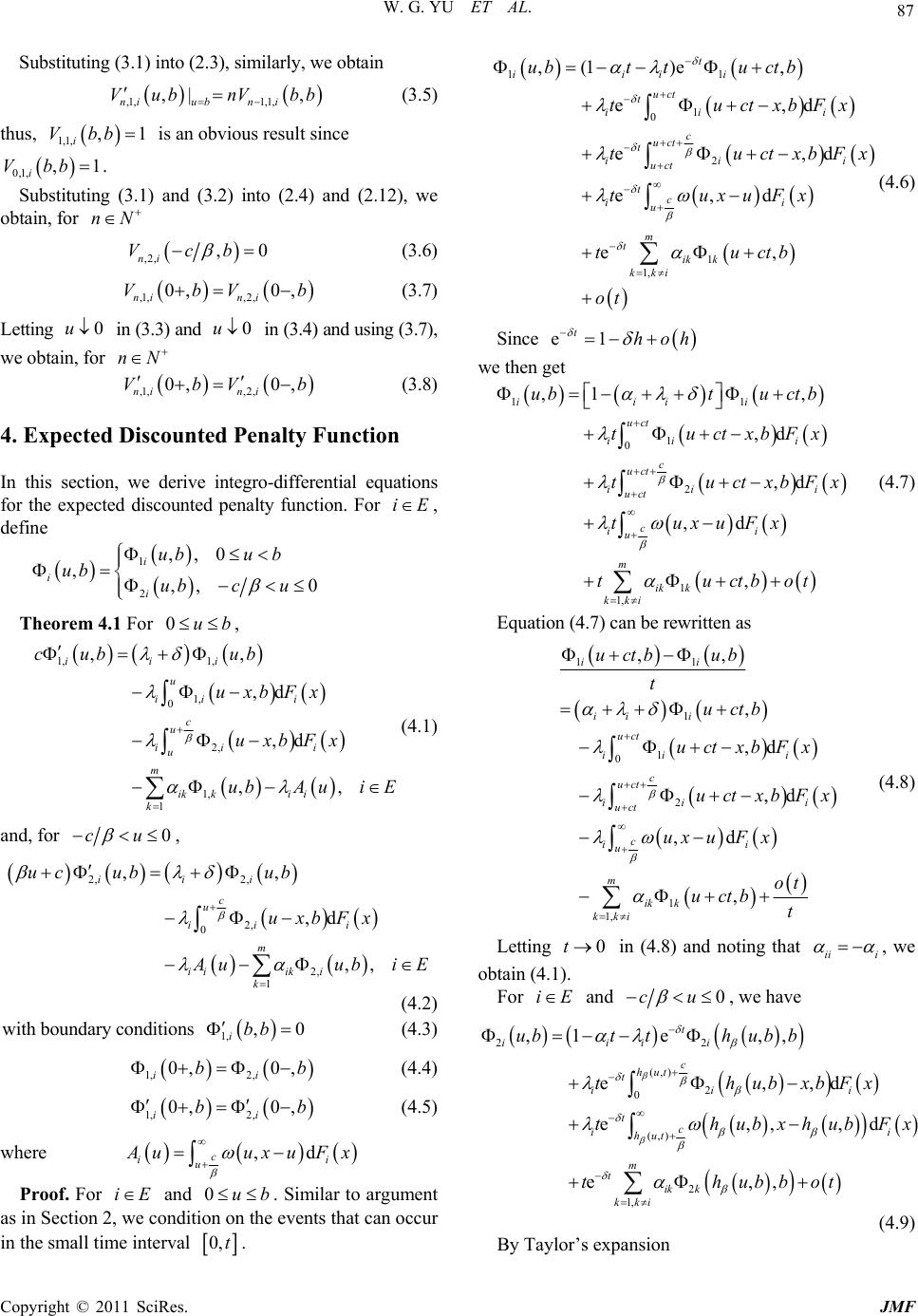 87 W. G. YU ET AL. Substituting (3.1) into (2.3), similarly, we obt ain ,1, 1,1, ,| , niubn i VubnVbb (3.5) thus, is an obvious result since 1,1, , i Vbb1 0,1,i,1Vbb. Substituting (3.1) and (3.2) into (2.4) and (2.12), we obtain, for nN ,2, , ni Vcb 0 b b (3.6) ,1, ,2, 0, 0, nin i VbV (3.7) Letting in (3.3) and in (3.4) and using (3.7), we obtain, for 0u0u nN ,1, ,2, 0, 0, nin i VbV (3.8) 4. Expected Discounted Penalty Function In this section, we derive integro-differential equations for the expected discounted penalty function. For iE , define 1 2 ,,0 ,,, 0 i i i ubu b ub ubc u Theorem 4.1 For , 0ub 1, 1, 1, 0 2, 1, 1 ,, ,d ,d ,, iii u ii i c u iii u m ikki i k cub ub uxbFx uxbFx ubA uiE (4.1) and, for 0cu , 2, 2, 2, 0 2, 1 ,, ,d ,, iii c u iii m iiik i k u cubub uxbFx uub iE (4.2) with boundary conditions 1, , ibb 0 b b (4.3) 1, 2, 0, 0, ii b (4.4) 1, 2, 0, 0, ii b (4.5) where ,d c ii u uuxuF x Proof. For and . Similar to argument as in Section 2, we condition on the events that can occur in the small time interval iE0ub 0,t. 11 1 0 2 1 1, ,(1 )e, e, e, e,d e, t iiii uct t ii i c uct t ii uct tc ii u m tik k kki ubttu ctb tuctxbF tuctxb tuxuFx tuctb ot d d i x Fx (4.6) Since e1 thoh we then get 11 1 0 2 1 1, ,1 , ,d ,d ,d , iiii uct ii i c uct ii uct c ii u m ik k kki ubtuctb tuctxbFx tuctxbF tuxuFx tuctbo i x t (4.7) Equation (4.7) can be rewritten as 11 1 1 0 2 1 1, ,, , ,d ,d ,d , ii ii i uct ii i c uct ii i uct c ii u m ik k kki uctb ub t uctb uctxbFx uctxbFx uxuFx ot uctb t (4.8) Letting in (4.8) and noting that 0tii i , we obtain (4.1). For iE and 0cu , we have 22 (,) 2 0 (,) 2 1, ,1 e,, e,,d e,,, e,, t iiii c hut t ii i tc ii hut m tik k kki ubtthub b thubxbF th ubxh ubFx thubbot d x (4.9) By Taylor’s expansion Copyright © 2011 SciRes. JMF 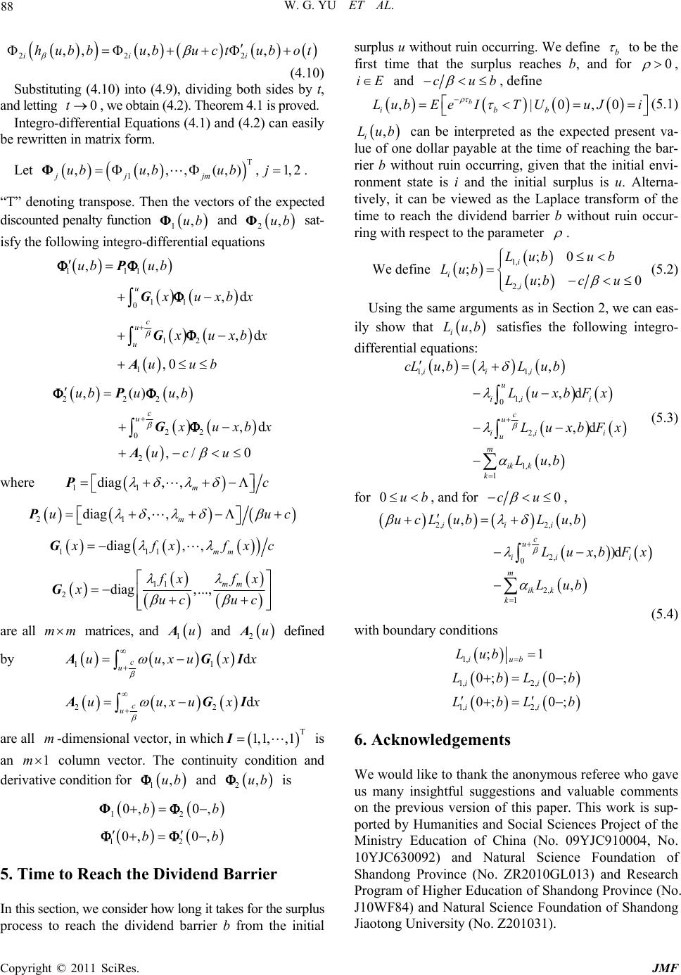 W. G. YU ET AL. 88 22 2 ,, ,, ii i hubbubuctub ot 1,2 (4.10) Substituting (4.10) into (4.9), dividing both sides by t, and letting , we obtain (4.2). Theorem 4.1 is proved. 0t Integro-differential Equations (4.1) and (4.2) can easily be rewritten in matrix form. Let . T 1 ,,,,(,), jj jm ubububjΦ “T” denoting transpose. Then the vectors of the expected discounted penalty function 1,ubΦ and 2,ubΦ sat- isfy the following integro-differential equations 111 11 0 12 1 ,, ,d ,d ,0 u c u u ub ub uxbx uxbx uub P G G A 222 22 0 2 ,(), ,d ,/0 c u ubuub uxbx uc u P G A where 11 diag,,mc P 21 diag,, m uu Pc 111 diag, , mm fxf xcG 11 2diag ,..., mm xf xuc uc Gx are all matrices, and and defined b y mm 1uA 2uA 11 ,dx c u uuuxIxAG 22 ,d c u uuxuxAGxI are all -dimensional vector, in whichm 1,1, ,1 I 2,ub is an column vector. The continuity condition and derivative condit i on for and is 1m 1,ub 12 0, 0, bbΦ 12 0, 0, bb 5. Time to Reach the Dividend Barrier In this section, we consider how long it takes for the surplus process to reach the dividend barrier b from the initial surplus u without ruin occurring. We define b to be the first time that the surplus reaches b, and for 0 , iE and cub , define ,|0 b ibb LubEeIT UuJi ,0 (5.1) , i Lub can be interpreted as the expected present va- lue of one dollar payable at the time of reaching the bar- rier b without ruin occurring, given that the initial envi- ronment state is i and the initial surplus is u. Alterna- tively, it can be viewed as the Laplace transform of the time to reach the dividend barrier b without ruin occur- ring with respect to the parameter . We define 1, 2, ;0 ;;0 i i i Lubub Lub Lub c u (5.2) Using the same arguments as in Section 2, we can eas- ily show that , i Lub satisfies the following integro- differential equations : 1, 1, 1, 0 2, 1, 1 ,, ,d ,d , iii u ii i c u iii u m ik k k cL ubL ub LuxbFx LuxbFx Lub (5.3) for 0ub , and for 0cu , 2, 2, 2, 0 2, 1 ,, ,)d , iii c u iii m ik k k ucL ubLub LuxbFx Lub (5.4) with boundary conditions 1, ;1 iub Lub 1, 2, 0; 0; ii LbL b 1, 2, 0; 0; ii LbL b 6. Acknowledgements We would like to thank the anonymous referee who gave us many insightful suggestions and valuable comments on the previous version of this paper. This work is sup- ported by Humanities and Social Sciences Project of the Ministry Education of China (No. 09YJC910004, No. 10YJC630092) and Natural Science Foundation of Shandong Province (No. ZR2010GL013) and Research Program of Higher Education of Shandong Province (No. J10WF84) and Natural Science Foundation of Shandong Jiaotong University (No. Z201 031). Copyright © 2011 SciRes. JMF 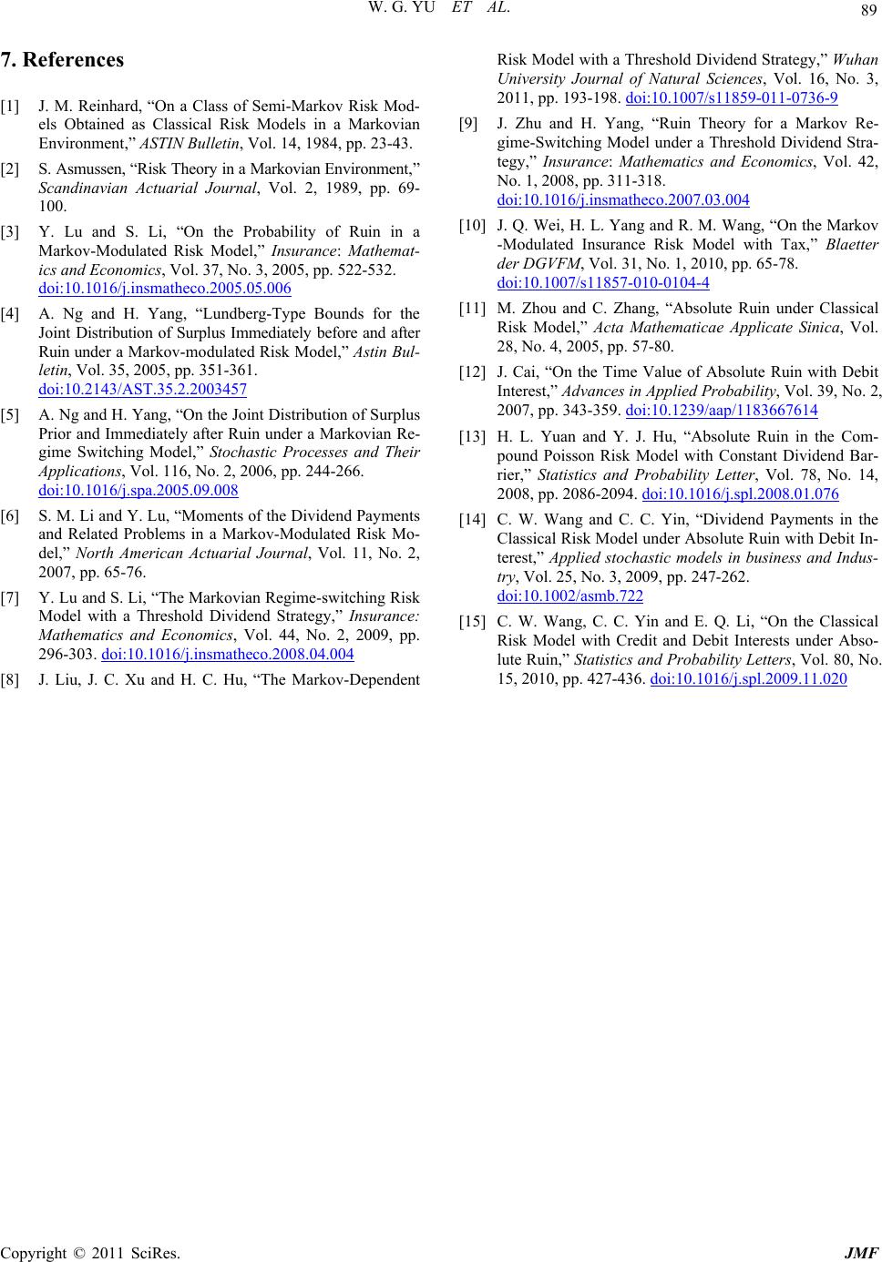 W. G. YU ET AL. Copyright © 2011 SciRes. JMF 89 7. References [1] J. M. Reinhard, “On a Class of Semi-Markov Risk Mod- els Obtained as Classical Risk Models in a Markovian Environment,” ASTIN Bulletin, Vol. 14, 1984, pp. 23-43. [2] S. Asmussen, “Risk Theory in a Markovian Environment , ” Scandinavian Actuarial Journal, Vol. 2, 1989, pp. 69- 100. [3] Y. Lu and S. Li, “On the Probability of Ruin in a Markov-Modulated Risk Model,” Insurance: Mathemat- ics and Economics, Vol. 37, No. 3, 2005, pp. 522-532. doi:10.1016/j.insmatheco.2005.05.006 [4] A. Ng and H. Yang, “Lundberg-Type Bounds for the Joint Distribution of Surplus Immediately before and after Ruin under a Markov-modulated Risk Model,” Astin Bul- letin, Vol. 35, 2005, pp. 351-361. doi:10.2143/AST.35.2.2003457 [5] A. Ng and H. Yang, “On the Joint Distribution of Surplus Prior and Immediately after Ruin under a Markovian Re- gime Switching Model,” Stochastic Processes and Their Applications, Vol. 116, No. 2, 2006, pp. 244-266. doi:10.1016/j.spa.2005.09.008 [6] S. M. Li and Y. Lu, “Moments of the Dividend Payments and Related Problems in a Markov-Modulated Risk Mo- del,” North American Actuarial Journal, Vol. 11, No. 2, 2007, pp. 65-76. [7] Y. Lu and S. Li, “The Markovian Regime-switching Risk Model with a Threshold Dividend Strategy,” Insurance: Mathematics and Economics, Vol. 44, No. 2, 2009, pp. 296-303. doi:10.1016/j.insmatheco.2008.04.004 [8] J. Liu, J. C. Xu and H. C. Hu, “The Markov-Dependent Risk Model with a Threshold Dividend Strategy,” Wuhan University Journal of Natural Sciences, Vol. 16, No. 3, 2011, pp. 193-198. doi:10.1007/s11859-011-0736-9 [9] J. Zhu and H. Yang, “Ruin Theory for a Markov Re- gime-Switching Model under a Threshold Dividend Stra- tegy,” Insurance: Mathematics and Economics, Vol. 42, No. 1, 2008, pp. 311-318. doi:10.1016/j.insmatheco.2007.03.004 [10] J. Q. Wei, H. L. Yang and R. M. Wang, “On the Markov -Modulated Insurance Risk Model with Tax,” Blaetter der DGVFM, Vol. 31, No. 1, 2010, pp. 65-78. doi:10.1007/s11857-010-0104-4 [11] M. Zhou and C. Zhang, “Absolute Ruin under Classical Risk Model,” Acta Mathematicae Applicate Sinica, Vol. 28, No. 4, 2005, pp. 57-80. [12] J. Cai, “On the Time Value of Absolute Ruin with Debit Interest,” Advances in Applied Probability, Vol. 39, No. 2, 2007, pp. 343-359. doi:10.1239/aap/1183667614 [13] H. L. Yuan and Y. J. Hu, “Absolute Ruin in the Com- pound Poisson Risk Model with Constant Dividend Bar- rier,” Statistics and Probability Letter, Vol. 78, No. 14, 2008, pp. 2086-2094. doi:10.1016/j.spl.2008.01.076 [14] C. W. Wang and C. C. Yin, “Dividend Payments in the Classical Risk Model under Absolute Ruin with Debit In- terest,” Applied stochastic models in business and Indus- try, Vol. 25, No. 3, 2009, pp. 247-262. doi:10.1002/asmb.722 [15] C. W. Wang, C. C. Yin and E. Q. Li, “On the Classical Risk Model with Credit and Debit Interests under Abso- lute Ruin,” Statistics and Probability Letters, Vol. 80, No. 15, 2010, pp. 427-436. doi:10.1016/j.spl.2009.11.020
|