Journal of Mathematical Finance, 2011, 1, 50-57
doi:10.4236/jmf.2011.13007 Published Online November 2011 (http://www.SciRP.org/journal/jmf)
Risk Aggregation by Using Copulas in Internal Models
Tristan Nguyen, Robert Danilo Molinari
Department of Economics, WHL Graduate School of Business and Economics, Lah r, Germany
Received August 17, 2011; revised October 9, 2011; accepted October 20, 2011
Abstract
According to the Solvency II directive the Solvency Capital Requirement (SCR) corresponds to the eco-
nomic capital needed to limit the probability of ruin to 0.5%. This implies that (re-)insurance undertakings
will have to identify their overall loss distributions. The standard approach of the mentioned Solvency II di-
rective proposes the use of a correlation matrix for the aggregation of the single so-called risk modules re-
spectively sub-modules. In our paper we will analyze the method of risk aggregation via the proposed appli-
cation of correlations. We will find serious weaknesses, particularly concerning the recognition of extreme
events, e.g. natural disasters, terrorist attacks etc. Even though the concept of copulas is not explicitly men-
tioned in the directive, there is still a possibility of applying it. It is clear that modeling dependencies with
copulas would incur significant costs for smaller companies that might outbalance the resulting more precise
picture of the risk situation of the insurer. However, incentives for those companies who use copulas, e.g.
reduced solvency capital requirements compared to those who do not use it, could push the deployment of
copulas in risk modeling in general.
Keywords: Solvency II, Risk Capital, Risk Measures, Risk Dependencies, Aggregation of Risks, Copulas
1. Introduction
The Solvency II directive of the European Commission
[1] focuses on an economic risk-based approach and
therefore obliges insurance undertakings to determine their
overall loss distribution function. The increasing complex-
ity of insurance products makes it necessary to consider
dependencies between the single types of risk to deter-
mine this function properly. Neglecting those dependencies
may have serious consequences underestimating the overall
risk an insurer is facing. On the other hand, assuming com-
plete dependency between risks may result in an overes
timate of capital requirements and therefore incur too high
capital costs for an insurance company. The Solvency II
draft directive acknowledges this fact and proposes rec-
ognition of dependencies by the use of linear correlations.
Reason is that correlations are relatively easy to under-
stand and to apply. However, the use of correlation re-
quires certain distributional assumptions which are inva-
lidated e.g. by non-linear derivative products and the
typical skew and heavy tailed insurance claims data.
Therefore aggregation of insurance risks via correlations
may neglect important information concerning the tail of
a distribution.
In contrast, copulas provide full information of de-
pendencies between single risks. Therefore they have be-
come popular in recent years. The copulas concept in an
insurance context was first introduced by Wang [2], who
discusses models and algorithms for the aggregation of
correlated risk portfolios. Frees and Valdez [3] provided
an introduction to the use of copulas in risk measurement
by describing the basic properties of copulas, their rela-
tionships to measures of dependence and several families
of copulas. Blum, Dias and Embrechts [4] discuss the use
of copulas to handle the measurement of dependence in
alternative risk transfer products. McNeil [5] presents
algorithms for sampling from a specific copula class which
can be used for higher-dimensional problems. Eling and
Toplek [6] analyze the influence of non-linear dependen-
cies on a non-life insurer’s risk and return profile.
As copulas allow the separate modeling of risks and the
dependencies between them, it will also be possible to ex-
plore the impact of (different) dependency structures on
the required solvency capital if they are used [7]. Differ-
ent dependency structures can be modeled on the one hand
through modified parameters of the copula function and
on the other hand through the choice of a completely dif-
ferent copula family. Following some recent contributions
[8,9], our aim is to give an overview over the concept of
copulas, to analyze and discuss their possible application

51 T. NGUYEN ET AL.
in the context of Solvency II and finally to make them
accessible to a wider circle of users. In this context we
would also like to discuss, if the new Solvency II direc-
tive forms an accurate concept for considering risk de-
pendencies or if further adjustments should be made.
Relating to that it will also be necessary to discuss de-
pendency ratios like the correlation coefficient but also
others (e.g. Spearman’s rank correlation).
We will therefore start with an overview over depen-
dency ratios. In Section 3 we will continue with the in-
troduction of copulas and illustrate different families and
types of copulas. After that we will briefly describe how
copulas and multivariate distributions can be determined
out of empirical data in Section 4. The paper will conti-
nue with an assessment of the presented dependence con-
cepts in Section 5 and end with a description and an as-
sessment of the consideration of risk dependencies in the
Solvency II framework in Section 6.
2. Dependency Ratios
Using the linear correlation coefficient is a very rudi-
mentary, but also simple way of describing risk depend-
encies in a single number. The linear correlation coeffi-
cient of real valued non-degenerate random variables X,
Y is defined by the following Equation (1):
 
 
,
,CovX Y XY
VarXVar Y
 , (1)
where ρ(X,Y) is the linear correlation coefficient of X and
Y, Cov(X,Y) = E[XY] – E[X]E[Y] is the covariance of X
and Y and Var(X) and Var(Y) are the finite variances of X
and Y.
In case of multiple dimensions the so called correlation
matrix needs to be applied. Equation (2) shows this sym-
metric and positive semi-definite correlation matrix:



 
11 1
1
,,
,
,,
n
nn

n
X
YX
XY
Y
X
YX






Y
n
(2)
i.e. .
 
,
, ,,1a,b
ab
ab
XYX Y  
The linear correlation coefficient (also called Pearson’s
linear correlation) measures only linear stochastic de-
pendency of two random variables. It takes values be-
tween –1 and 1, i.e. –1 ≤ ρ(X,Y) ≤ +1. However, perfectly
positive correlated random variables do not necessarily
feature a linear correlation coefficient of 1 and perfectly
negative correlated random variables do not necessarily
feature a linear correlation coefficient of –1. Random va-
riables that are strongly dependent may also feature a lin-
ear correlation coefficient which is according to amount
close to 0.
Two pairs of random variables with a certain linear
correlation coefficient may actually have a completely dif-
ferent dependence structure. Figure 1 which shows reali-
zations of two pairs of random variables (X1 and X2 re-
spectively X1 and X3) that both have the same linear cor-
relation, clearly illustrates this.
The covariance and thus also the linear correlation be-
tween independent random variables is zero. However, if
the linear correlation coefficient between two random
variables is near zero, it can actually exist a high correla-
tion between them. Linear correlation is a natural de-
pendency ratio for elliptically distributed risks. If used
for random variables that are not distributed elliptically,
linear correlation can lead to wrong results. Extreme events
with high losses can be severely underestimated by using
the linear correlation as a measure for dependencies be-
tween risks [10]. Modeling major claims often requires
the use of distributions with infinite variances for which
the linear correlation coefficient is not defined. In addition
linear correlation is not invariant concerning non-linear
monotone transformations which may cause problems
when an amount of loss is converted into a loss payment.
Two other ratios for measuring risk dependencies are e.g.
Spearman’s rank correlation and Kendall’s τ. However,
they do also not fully inform on dependencies between
risks, but rather compress all information into a single
number. The coefficient of tail dependence (important
for non-life insurers modeling extreme events) for two
random variables X and Y describes the likelihood of Y
taking an extreme value on condition that X also takes an
extreme value. This also means that the coefficient of tail
dependence does not provide full information on the de-
pendence structure between random variables. The fol-
lowing Equations (3)-(5) show the three dependency
ratios:




,,
SXY
X
YFXFY  , (3)
Figure 1. Dependence structure between random variables
X1 and X2 respectively X1 and X3 [11].

T. NGUYEN ET AL.
52


0

1
where Fx is the distribution function of X, Fy is the dis-
tribution function of Y and F would be the joint distribu-
tion function.
 



1212
1212
,
0
XYP XXYY
PXX YY
 
 
(4)
where (X1,Y1) and (X2,Y2) are two independent and iden-
tically distributed pairs of random variables from F.
 

1
1
,lim |
YX
XYPY FXF





 , (5)
on the condition that this limit


0, 1   exists.
3. Copulas
In contrast, copulas provide full information on the de-
pendency structure between risks. Copulas allow the se-
paration of the joint marginal distribution function into a
part that describes the dependence structure and parts
that describe the marginal distribution functions.
The Copula is a multivariate distribution function with
margins that are uniformly distributed on [0,1] and was
defined by Sklar [12]:

111
,, ,, 
nn
CuuPU uUu

n
, (6)
where C( ) is the copula, (U1,,Un)T with Ui ~ U(0,1)
for all i = 1,, n a vector of random variables and
(u1,,un)T [0,1]n realizations of (U1,,Un)T. 
The risk modeling process with copulas consists of
two steps. First one has to determine the marginal distri-
bution of every single risk component. Secondly the de-
pendence structure between these risk components has to
be determined via the copula function. In order to obtain
the joint distribution function the n single risks Xi have
then to be transformed each into a random variable Ui that
is uniformly distributed on [0,1] by using using the cor-
responding marginal distribution Fi


iii
UFX. (7)
We obtain the multivariate distribution function by in-
serting these transformed random variables into the co-
pula function:
 

 
11 11
,, ,, ,,
nn

nn
F
xx Cuu CFxFx (8)
In case of continuous and differentiable marginal dis-
tributions and a differentiable copula the joint density is:












111 11
,, ***,,
nnnnn
f
xx fxfxcFx Fx 
,
(9)
where fi(xi) is the respective density for distribution func-
tion Fi and


1
1
1
,,
,,
n
n
n
n
Cu u
cu uuu




the density of the copula.
In this way we can derive a multivariate distribution
function out of specified marginal distributions and a co-
pula that contains information about the dependence
structure between the single variables. But also the oppo-
site holds: A copula can be determined out of the inverse
of the marginal distributions and the multivariate distri-
bution function.
The most important copula families are (the bands in
which the dependencies are stronger or weaker differ):
 Elliptical copulas
o Gaussian copulas
o Student copulas
 Archimedean copulas
o Gumbel copulas
o Cook-Johnson copulas
o Frank copulas
Equation (10) shows the definition of the Gaussian
copula:

  


11
11
,, ,,
Gau n
nn
Cu uuu


 , (10)
n


is the distribution function of the n-variate standard
normal distribution with correlation matrix ρ an 1 d


is the inverse of the distribution function of the univari-
ate standard normal distribution. The dependency in the
tails of multivariate distributions with a Gaussian copula
goes to zero [13], which means that the single random
variables of the joint distribution function are almost
independent in case of high realizations. Insurance risks
feature in most cases weak dependency for lower values
and strong dependency for higher realizetions. From this
perspective the Gaussian copula does not provide a pro-
per basis for modeling insurance risks.
In contrast, Student copulas do not feature independ-
ency in the tails of a distribution [7]. Equation (11) shows
how they can be defined:

  


11
,1 ,1
,, ,,
Stu n
nv n
Cuu ttutu
 

, (11)
where ν is the number of degrees of freedom, ,
n
t


the
distribution function of the n-variate Student distribution
with ν degrees of freedom and a correlation matrix of ρ
and 1
t


the inverse of the distribution function of the
univariate Student distribution with ν degrees of freedom.
The Figures 2 and 3 show the densities for both the
bivariate Gaussian and the bivariate Student copula. An-
other class of copulas is given by the Archimedean
copulas which can be written in the form:

  


1
11
,,
nn
Cu uuu  

, (12)
for all 1 0,,
n
uu1

 and

is some continuous
function (called the generator) satisfying:

53 T. NGUYEN ET AL.
Figure 2. Density of a Gaus s ian copula (correlation ρ of 0.7).
Figure 3. Density of a student copula (correlation ρ of 0.7).
1) ;

10  
2)

is strictly decreasing and convex and;
3) is completely monotonic on

.
1


0, 
Among others the Gumbel copulas belong to the Ar-
chimedean copulas. Similarly to the Student copulas they
are tail dependent, however, not in both the upper and
the lower tail, but only in the upper one (see Figure 4).
Therefore they are adequate for modeling extreme events:
On the one hand stress scenarios [14] (with high losses
and high dependence) can be captured and on the other
hand common (lower) losses which in general appear
independent can be modeled. Equation (13) shows the
formula for Gumbel copulas:

 

1
1ln
1,, e
ni
iu
Gum
n
Cuu











 , (13)
β ≥ 1 is a structural parameter. β = 1 leads to a multi-
variate distribution of independent random variables. Only
in this case the Gumbel copula is independent in the up-
per tail.
Cook-Johnson copulas represent another Archimedean
copula. Contrary to the Gumbel copulas they are tail de-
pendent only in the lower tail (see Figure 5). Therefore
they perform good results if used for modeling yields on
shares [15]. The following equation describes the Cook
Johnson copulas:


1
11
,, 1






CJ
nn
Cuuuun, (14)
β > 0 is a structural parameter.
The third type of Archimedean copulas presented in
this paper is the Frank copula. This type of copulas is
completely tail independent [16,17]. The dependence
structure given by a copula of this type is similar to one
represented by a Normal copula even though the dependence
Figure 4. Gumbel copula with structural parameter β = 2.
Figure 5. Cook-Johnson copula with structural parameter
β = 2.

T. NGUYEN ET AL.
54
in the tail is even lower (see Figure 6). Equation (15)
shows the definition of Frank copulas:


 

1
11
e1e1
1
,, ln1
e1
n
u u
Fra
nn
Cu u
 


 





 











,
(15)
β > 0 is a structural parameter.
4. Determination of Copulas and
Multivariate Distributions
Using the concept of copulas for capturing dependencies
between risks in an insurance company, first of all the
corresponding copulas have to be determined. Two al-
ternative approaches for achieving this are parametric
and non-parametric approaches. Using a parametric ap-
proach means to first determine the respective type of
copula [10]. As shown above the various types of copu-
las describe a different type of dependence structure each.
Therefore it is necessary to choose that type of copulas
that best fits the actual dependence structure. We can
follow a procedure for the bivariate case established by
Genest and Rivest [18] which uses the dependency ratios
for identifying a type of Archimedean copula that fits the
observations. The procedure is carried out in 3 steps [19]:
1) Estimation of Kendall’s τ out of the observations
(X11, X21),, (X1n, X2n).
2) Define an intermediate random variable Zi = F(X1i,
X2i) with distribution function K. Genest, C. and Rivest,
L.-P. (1993) showed that the following statement holds:
 

z
Kz zz


 (16)
Figure 6. Frank copula with structural parameter β = 2.


z  is the generator of (and therefore determines) an
Archimedean copula.
Construct a non-parametric estimate of K:
a) Define pseudo observations Zi = {number of (X1j,
X2j) such that X1j < X1i and X2j < X2i}/(n – 1) for i = 1,,n.
b) Estimate of K is Kn(z) = {number of Zi ≤
z}/{number of Zi}.
3) Construct parametric estimate of K using the rela-
tionship of (16): Use the estimate of Kendall’s τ from
Step 0 and the given relation between Kendall’s τ and the
generator of a specific type of a copula


z 
to come
to a parametric estimate of K.
Repeat step three with generators for different types of
copulas. At the end choose that type of copula where the
parametric estimate of K most closely resembles the
non-parametric estimate of K calculated in Step 0.
Once the type of copula is chosen, the parameters of
the copula have to be determined as a best-estimate. This
can be achieved in course of the estimation of the pa-
rameters of the marginal distribution by using the maxi-
mum likelihood method [16]. Since one of the advan-
tages of using copulas is the separate estimation of the
marginal distributions and the dependence structure also
a two-step approach can be applied: in the first step the
parameters of the marginal distributions are estimated and
in a second step those of the copula.
Using the non-parametric approach means determining
an empirical copula out of the empirical data and therefore
not determining a specific copula type in advance [10].
5. Assessment
In the previous sections we provided an overview over
dependency ratios and copulas, two—very different—con-
cepts for describing dependencies between risks. Both of
these concepts will be assessed in the following. How-
ever, first we will introduce 5 criteria that dependency
ratios should meet.
5.1. Criteria for Dependency Ratios
The following five criteria are desirable for a dependency
ratio. Therefore we will first explain the criteria and af-
terwards match the introduced dependency ratios with
them. If δ( ) is a dependency ratio, the criteria can be
described as the following:
1) symmetry: δ(X,Y) = δ(Y,X);
2) standardization: –1 ≤ δ(X,Y) ≤ 1;
3) conclusion based on and on co- and countermono-
tonity;
a) δ(X,Y) = 1

X,Y are comonotone;
b) δ(X,Y) = –1

X,Y are countermonotone;

55 T. NGUYEN ET AL.
4) Invariance with regard to strictly monotone trans-
formations: For a transformation strictly mono-
tone on the codomain of X the following holds:
:T
a) δ(T(X),Y) = δ(X,Y), if T is strictly monotonic in-
creasing;
b) δ(T(X),Y) = –δ(X,Y), if T is strictly monotonic de-
creasing;
5) conclusion based on and on independence
δ(X,Y) = 0 X,Y are independent. 
The first criterion is desirable for dependency ratios
because otherwise the resulting dependency ratio would
depend on the order of the considered risks. If a depend-
ency ratio fulfills the second criterion, this will lead to an
unique measure which makes dependencies between pairs
of random variables comparable. Conclusion based on and
on co- and countermonotonity helps to immediately de-
tect strongly dependent random variables.
Invariance with regard to strictly monotone transfor-
mations is mainly important if the dependency ratio is
used for practical applications. If a random variable X is
transformed into another variable T(X) using a strictly
monotone function T, the dependence structure between
X and a second random variable Y will be the same as the
dependence structure between T(X) and Y. Therefore also
the dependency ratio should take on the same value for
T(X) and Y as for X and Y. The last criterion makes sure
that also independency between random variables can be
detected.
5.2. Assessment of the Introduced Concepts
First, we want to assess the dependency ratios. The most
popular of those—the Pearson linear correlation coeffi-
cient—only fulfills the first two criteria of the above
mentioned five. From this point of view it is inferior com-
pared to Spearman’s rank correlation and Kendall’s τ which
fulfill the first four of the mentioned five criteria. Further-
more, the Pearson linear correlation coefficient is defined
only if the variances of the random variables are finite.
Another advantage of both Spearman’s rank correla-
tion and Kendall’s τ is that they do not only measure the
linear dependency between random variables, but also
the monotone dependence in common [13]. Their calcu-
lation may be sometimes easier, but sometimes more
difficult than the calculation of the Pearson linear corre-
lation coefficient. Using e. g. multivariate normal distri-
butions or multivariate Student distributions the calculation
of the momentum based linear correlation coefficient is
easier. However, if we consider multivariate distributions
that have a dependence structure represented by a Gum-
bel copula, the calculation of Spearman’s rank correla-
tion and Kendall’s τ might be easier.
The coefficient of tail dependence introduced in Section
2 should not be compared to one of the above mentioned
three dependency ratios, since it focuses only on the de-
pendency in the tails of a distribution. It should therefore be
applied if it is required by the respective problem. This is
the case mainly if extreme events are modeled. Therefore
we think that matching the five criteria with the coeffi-
cient of tail dependence is not reasonable.
Copulas can be used to model multivariate distributions
which fully describe the dependence structure. In this way a
whole picture of the aggregate risk an insurer is facing.
The fact that a given copula implies a certain value for
the correlation, but in general not the other way around,
makes clear that a copula contains much more information
than a dependency ratio. Especially, when dependencies are
not linear, but are located in the tails, risk could be sig-
nificantly underestimated if incomplete information is
considered.
From a technical point of view copulas offer the op-
portunity to first model the marginal distribution func-
tions representing the single risks and in a second step
modeling the dependence structure independently from
the single risks. Furthermore, similar to Spearman’s rank
correlation and Kendall’s τ copulas are invariant with
regard to strictly monotone transformations [11]. A fur-
ther technical advantage of using copulas instead of di-
rectly modeling multivariate distributions is that the mar-
ginal distribution function can then be of any type, whe-
reas if the multivariate distribution function was directly
modeled, each of the marginal distribution functions would
have to be of the same type. Besides, directly modeling
the multivariate distribution function presumes that a
dependency ratio is given and therefore once more allows
only the use of only a ratio as a dependency measurement.
In summary, we can say that the concept of copulas is
clearly superior with regard to the quality of estimating
dependencies between risks. Even though ratios currently
have advantages in their practical usage—if the usage of
copulas becomes more popular in future, these advan-
tages of dependency ratios will be likely to disappear.
All in all we can say that since dependency ratios do
not provide a complete picture of the actual situation
with regard to risk dependencies, therefore provide sig-
nificant less information and finally may lead to an un-
derestimation of the actual risk of an insurance company,
copulas should be used to describe dependencies between
risks in an insurance company if possible. Particularly
for the option of introducing an internal risk model the
application of copulas seems to be suitable.
6. Solvency II
6.1. Consideration of Risk Dependencies in
Solvency II
According to the new European solvency system (Solvency

T. NGUYEN ET AL.
56
II) insurance undertakings will have to determine the so
called Solvency Capital Requirement (SCR) which re-
flects the amount of capital that is necessary to limit the
probability of ruin to 0.5%. That implies that they will
also have to determine their overall loss distribution fun-
ction. Hereby at least the following risks have to be con-
sidered [1]:
• non-life underwriting risk;
• life underwriting risk;
• health underwriting risk;
• market risk;
• credit risk;
• operational risk.
Insurers will be able to either use a standard approach
or to determine the Solvency Capital Requirement or parts
thereof by the use of an internal model. In the latter case
the internal model has to be approved by the supervisory
authorities. Using the standard approach, the SCR is the
sum of the Basic Solvency Capital Requirement, the ca-
pital requirement for operational risk and the adjustment
for the loss-absorbing capacity of technical provisions
and deferred taxes.
The Basic Solvency Capital Requirement consists at
least of a risk module for non-life underwriting risk, for
life underwriting risk, for health underwriting risk, for
market risk and for counterparty default risk each. These
risk modules have to be split into sub-modules [1]. The
sub-modules shall be aggregated using the same approach
as for the aggregation of the risk modules that is descri-
bed in the following.
After having been determined, the risk modules have
to be aggregated. The Solvency II directive clearly states
that for the standard approach this has to be done by us-
ing correlations and the following Equation (17):
,
,**
 ij ij
ij
BSCRSCRSCR , (17)
BSCR is the Basic Solvency Capital Requirement, SCRi
respectively SCR j are risk-modules i respectively j and
ρi,j is the correlation between them.
Table 1 shows the correlation matrix for aggregating
risk modules in Solvency II, where i,j = 1: risk module
for market risk, i,j = 2: risk module for counterparty de-
fault risk, i,j = 3: risk module for life underwriting risk,
i,j = 4: risk module for health underwriting risk, i,j = 5:
sk module for non-life underwriting risk.
6.2. ules with
Regard to Risk Dependencies
capital to the Basic Solvency Capital Re-
qu
for small and medium-sized insurance un-
de
ncies and that other dependency ratios should
be preferred.
Table 1. Correlation matrix for aggregating risk modules in Solvency II.
ri
Assessment of the Solvency II R
On a first level the Basic Solvency Capital Requirement,
the capital requirement for operational risk and the ad-
justment for the loss-absorbing capacity of technical pro-
visions and deferred taxes have to be aggregated. This is
done simply by adding the capital requirements which
assumes that those risks are fully dependent. However,
the assumption that full dependence between e.g. the op-
erational risk and the risks covered by the BSCR is not
realistic and therefore the result for the SCR will be too
high. However, the amount of solvency capital for the
operational risk is limited [1]. Against this background we
think that it would be sensible to only consider the op-
erational risk qualitatively like Switzerland has decided
in the Swiss Solvency Test instead of simply adding an
amount of
irement.
The Solvency II framework closely recognizes depen-
dencies at least in the calculation of the BSCR. However,
the standard approach uses the concept of linear correla-
tions to consider dependencies between the risk modules
and not copulas which is certainly due to the application
of the proportionality principle in the Solvency II direc-
tive which has to assure that the regulation is not too
burdensome
rtakings.
Another shortcoming of the regulation set is that the
given values for the correlations which are shown in Ta-
ble 1 seem to be highhanded and do not reflect the spe-
cific situation of an insurance company. Moreover, we
have shown in Section 5 that some serious underestima-
tions may occur if linear correlations are used for meas-
uring depende
j = 1: market risk underwriting risk underwriting risk
j = 5: non-life
underwriting risk
j = 2: counterparty j = 3: life j = 4: health
ji,

default risk
i = 1: market risk 1 0.25 0.25 0.25 0.25
i = 2: counterparty default risk 0.
0
k 0.25
251 0.25 0.25 0.5
i = 3: life underwriting risk 0.25 .251 0.25 0
i = 4: health underwriting ris0.25 0.25 1 0
i = 5: non-life underwriting risk0.25 0.5 0 0 1

T. NGUYEN ET AL. 57
However, the Solvency IIves the possi-
bility to apply also the concto capture de-
odel. Tsupervisory aut
mp
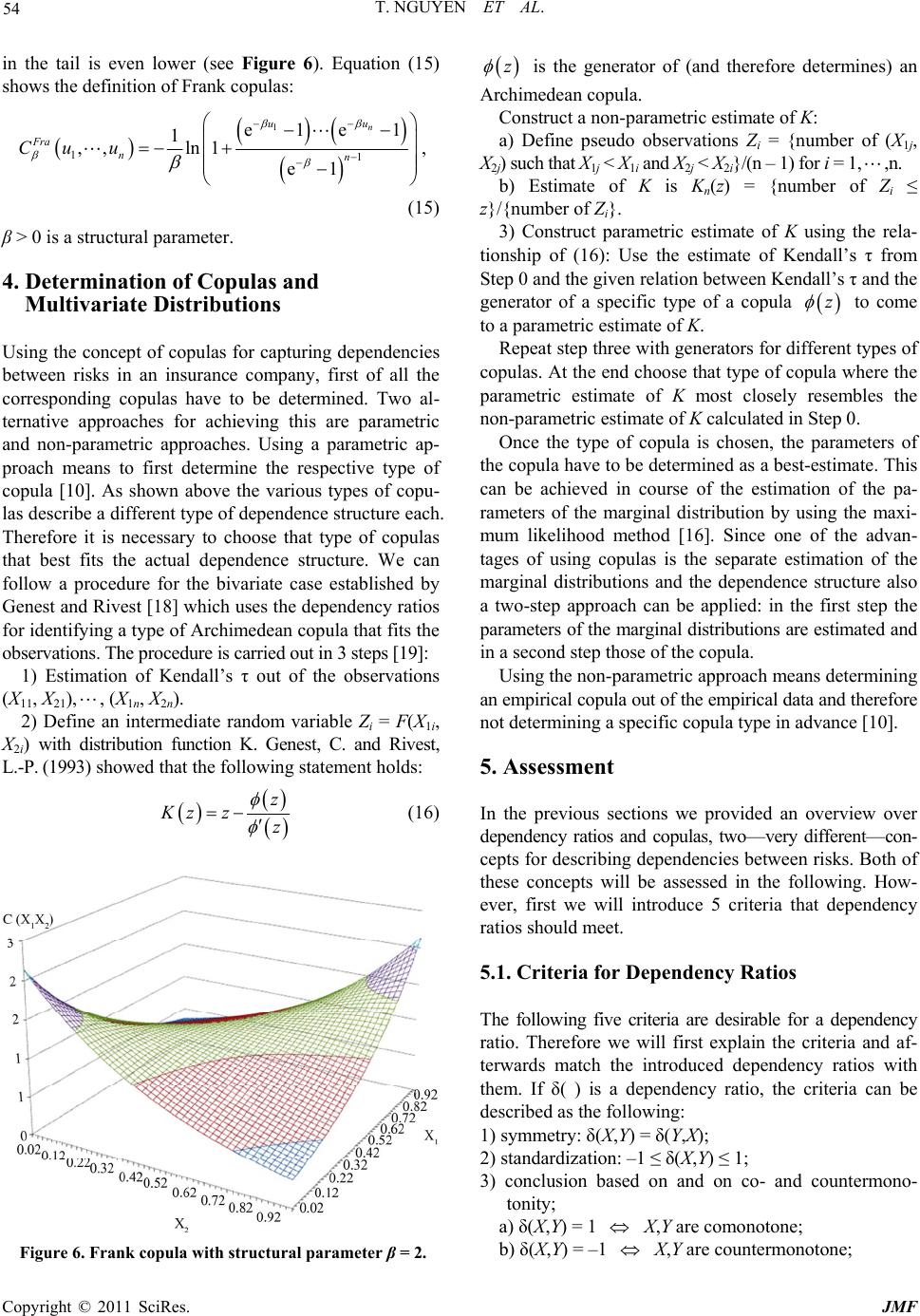
a
ers which measure the dependencies
be
ve
us
pean Par-
liament and of the Council on the Taking-Up and Pursuit
ss of Insurance and Reinsurance,” 2009.
nsilium.europa.eu/pdf/en/09/st03/
Valdez, “Understanding Relation-
T of
78, No. 6, 2007, pp.
doi:10.1080/00949650701255834
framework gi
ept of copulas
pendencies in an internal m
ties may even require the co
he
anies to apply an inter-
ho-
ri
nl model for calculating the Solvency Capital Require-
ment, or a part thereof, if it is inappropriate to calculate
the Solvency Capital Requirement using the standard ap-
proach [1]. That means that if the approach for consider-
ing dependencies that is given in the standard model does
not lead to a realistic picture of the actual risk situation
of the company, the supervisory authorities may oblige
the company to use a more sophisticated way for captur-
ing dependencies.
Since the Solvency II framework does not use copulas
in the standard formula for reason of the proportionality
principle, we recommend that Solvency II should at least
reward those insur
tween their risks in a more sophisticated way. This could
be achieved either by reducing the SCR for those insur-
ers or the other way around by imposing higher require-
ments on companies which use the rudimental standard
approach. That would also be justifiable from an econo-
mical point of view: Companies that use linear correlations
may severely underestimate their overall risk and should
therefore be protected by higher capital requirements.
It would also make sense and give additional incen-
tives to explicitly mention the concept of copulas in the
directive and to rework the standard formula once the de-
velopment in multivariate modeling allows the effecti
e of copulas also for smaller insurance companies [20].
Moreover, we have discovered that the given correlations
do not seem to reflect an actual average of the insurance
industry. So, if correlations are used, they should at least
be actually measured in the insurance industry.
7. References
[1] European Commission, “Directive of the Euro
of the Busine
http://register.co
st03643-re06.en09.pdf
[2] S. Wang, “Aggregation of Correlated Risk Portfolios:
Models and Algorithms,” Proceedings of the Casualty
Actuarial Society, Vol. 85, 1998, pp. 848-939.
[3] E. W. Frees and E. A.
ships Using Copulas,” North American Actuarial Journal,
Vol. 2, No. 1, 1998, pp. 1-25.
[4] P. Blum, A. Dias and P. Embrechts, “The AR De-
pendence Modeling: The Latest Advances in Correlation
Analysis,” In: M. Lane, Ed., Alternative Risk Strategies,
Risk Books, London, 2002.
[5] A. J. McNeil, “Sampling Nested Archimedean Copulas,”
Journal of Statistical Computation and Simulation, Vol.
567-581.
[6] M. Elng and D. Toplek, “Modeling and Man
Nonlinear Dependencies-Copulas in Dynamic Financial
iagement of
Analysis,” Journal of Risk and Insurance, Vol. 76, No. 3,
2009, pp. 651-681.
doi:10.1111/j.1539-6975.2009.01318.x
[7] A. Tang and E. A. Valdez, “Economic Capital and the
Aggregation of Risks using Copulas,” 2006.
http://www.ica2006.com/Papiers/282/282.pdf
[8] A. Patton, “Copula-Based Models for Financial Time
Series,” In: T. G. Andersen, R. A. Davies, J.-P. Kreiss
and T. Mikosch, Ed., Handbook of Financial Time Series,
Springer, Berlin, 2009, pp. 767-785.
doi:10.1007/978-3-540-71297-8_34
[9] C. Genest, M. Gendron and M. Bourdeau-Brien, “The
Advent of Copulas,” European Journal of Finance, Vol.
15, No. 7-8, 2009, pp. 609-618.
doi:10.1080/13518470802604457
[10] G. Szegö, “Measures of Risk,” Journal of Banking and
Finance, Vol. 26, No. 7, 2002, pp. 1253-1272.
doi:10.1016/S0378-4266(02)00262-5
[11] D. Pfeifer, “Möglichkeiten und Gren
tischen Schadenmodellierung,” Zeitsc
zen der mathema-
hrift für die gesam-
à n Dimensions et Leurs
de Statistique de l’Un-
rrelation
nt: Properties and
zum
te Versicherungswissenschaft—German Journal of Risk
and Insurance, Vol. 92, No. 4, 2003, pp. 665-696.
[12] M. Sklar, “Fonctions de Répartition
Marges,” Publications de l’Institut
iversité de Paris, No. 8, 1959, pp. 229-231.
[13] P. Embrechts, A. McNeil and D. Straumann, “Co
and Dependence in Risk Manageme
Pitfalls,” 2002.
http://www.math.ethz.ch/~strauman/ preprints/pitfalls.pdf
[14] H.-J. Zwiesler, “Asset-Liability-Management—Die Ver-
sizcherung auf dem Weg von der Planungsrechnung
Risikomanagement,” In: K. Spremann, Ed., Versicherun-
gen im Umbruch—Werte Schaffen, Risiken managen, Kun-
den gewinnen, Springer, Berlin, 2005, pp. 117-131.
[15] T. Ané, T. and C. Kharoubi, “Dependence Structure and
Risk Measure,” Journal of Business, Vol. 76, No. 3, 2003,
pp. 411-438. doi:10.1086/375253
[16] M. Junker and A. May, “Measurement of aggregate risk
with copulas,” Econometrics Journal, Vol. 8, No. 3, 2005,
pp. 428-454. doi:10.1111/j.1368-423X.2005.00173.x
[17] G. G. Venter, “Tails of Copulas,” Proceedings of the Ca-
sualty Actuarial Society, Vol. 89, No. 171, 2002, pp. 68-113.
[18] C. Genest and L.-P. Rivest, “Statistical Inference Proce-
dures for Bivariate Archimedean Copulas,” Journal of the
American Statistical Association, Vol. 88, No. 423, 1993,
pp. 1034-1043. doi:10.2307/2290796
doi:10.1111/j.1539-6975.2009.01310.x
[19] E. W. Frees and E. A. Valdez, “Understanding Relation-
ships Using Copulas,” North American Actuarial Journal,
Vol. 2, No. 1, 1998, pp. 1-25.
[20] P. Embrechts, “Copulas: A Personal View,” Journal of
Risk and Insurance, Vol. 76, No. 3, 2009, pp. 639-650.