Theoretical Economics Letters, 2011, 1, 129-133
doi:10.4236/tel.[phone] Published Online November 2011 (http://www.SciRP.org/journal/tel)
Poverty Indices Revisited
Eugene Kouassi1, Pierre Mendy2, Diaraf Seck2, Kern O. Kymn3
1Resource Economics, West Virginia University, Morgantown, USA
2Faculty of Economics, University o f Cheick Anta Diop (UCAD), Dakar, Senegal
3Division of Finance a nd Eco nomi c s, West Virginia University, Morgantown, USA
Received September 13, 2011; revised October 19, 2011; accepted Octob er 28, 2011
Abstract
In this paper, a new optimization-based approach to constructing a poverty index is considered. From a gen-
eral perspective, first and second order conditions based on a general poverty intensity function are derived.
Then using specific intensity functions defined by [1,3] respectively, we specify related necessary and suffi-
cient conditions and the underlying poverty indices. An extension based on a large class of intensity function
is also investigated.
Keywords: A General Poverty Index, Necessary and Sufficient Conditions, Other Poverty Indices, Poverty
Intensity Functions
1. Introduction
How poverty is measured is a central topic in economic
and policy analyses. This paper contributes to the litera-
ture on this topic by providing methods for measuring
poverty in a static environment. In particular, one can
define a general poverty index and show that the existing
ones are some special cases of a more general index. An
extension is also proposed.
The remainder of the paper is organized as follows: a
general approach to constructing a poverty index is con-
sidered in Section 2. In particular; necessary as well as
sufficient conditions to determine the number of poor
persons are derived. In Section 3 based on specific inten-
sity functions, conditions to determine the number of poor
persons are specified. In Section 4, an extension based on
a more general poverty intensity function is proposed.
Finally, some concluding remarks are presented in Sec-
tion 5.
2. A General Approach to Construct A
Poverty Index
2.1. The Problem
In general poverty issue can be seen as an optimization
problem of the so called average intensity poverty func-
tion defined as . Specifically, the prob-
lem is to minimize a constrained program,

.: Q



2
1
Min
s.t Q
i
i
Y
Yr





 (1)
where r is a given strictly positive value which
represents the level richness of the individuals and
i is the income of individual . The above minimiza-
tion program is also equivalent to,
Q
Y i


*
Min ,
s.t ,Q
Y
Y










(2)
where represe n ts th e L ag r an g ian an d


the Lagrange
multipliers. Equation (2) can be solved to determine the
number of poor persons, .
Q
2.2. Solution
To solve the above minimization program, first and sec-
ond order conditions are required.
Theorem 1 Necessary Cond ition
A necessary condition to get a critical point to problem
(1) or (2) is that,


2
1
,1,,
i
i
Q
ii
Y
Y
Yr i
Y
Y



 
 




Q (3)

Proof: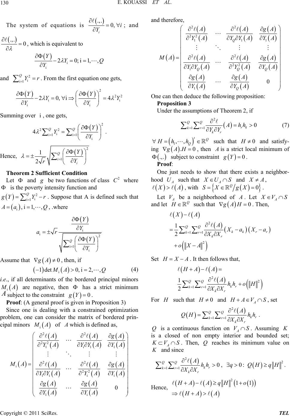

E. KOUASSI ET AL.
130
The system of equations is

.,. 0,
i
i
Y


; and

.,. 0



, which is equivalent to

i
i
20;i1,,
YYQ
Y

 

and . From the first equation one gets,
2
i
i1
QY

r
 
2
22
i
ii
20,i 4
YY
Y
YY

  
 


 i
Y 
Summing over , one gets,
i

2
22
i
i1i1 i
4QQ
Y
YY 

 



 .
Hence,

2
1
1
2
Q
ii
Y
Y
r



 



Theorem 2 Sufficient Condition
Let and

g
be two functions of class where
is the poverty intensity function and
2
C


2
i
i1
Q
g
YY




i,i 1,,
r. Suppose that A is defined such that
A
aQ, .where


i
i2
i1 i
Q
Y
Y
ar Y
Y




 




Assume that , then, if

0gA
 
i
1det0,i2, ,
M
AQ
(4)
i.e., if all determinants of the bordered principal minors

i
M
A are negative, then

has a strict minimum
subject to the constraint
A


gY 0.
Proof: (A general proof is given in Proposition 3)
Since one is dealing with a constrained optimization
problem, one can consider the matrix of bordered prin-
cipal minors

i
M
A of
A
which is defined as,


















22
22 i1 1
1
22
i
22
1i ii
1i
0
A
AgA
YY AY A YA
MA
A
AgA
YYA YAYA
gA gA
YA YA



 







 









 





and therefore,




  










22
22 111
22
22
1
1
0
Q
QQ
Q
Q
A
AgA
YYAYA YA
MA
A
AgA
YY AY A YA
gA gA
YAY A



  






  









 



One can then deduce the following proposition:
Proposition 3
Under the assumptions of Theorem 2, if

2
11 0
QQ
rk
krkr
Ahh
YY



  (7)


1,, tQ Q
Hh h  such that and satisfy-
ing 0H


.0gAH

, then
A
is a strict local minimum of


.,. subject to constraint .

gY 0
Proof:
One just needs to show that there exists a neighbor-
hood such that
A
UA
X
US

 and
X
A,




X
A, with



0X
Q
SX g

.
Let be a neighborhood of
A
V
A
. Let A
X
VS


and let Q
H

 such that . Then,

0gAH





 

2
11
2
1
2
QQ
kk rr
kr kr
XA
A
X
aXa
XX
oXA









Set
H
XA

. It then follows that,






22
11
1
2
QQ
kr
kr kr
HA A
Ahho H
XX

 





For
H
such that 0H

and A
H
AV S , set
 
2
11
QQ
kr
kr kr
A
QH hh
XX



 .
Q is a continuous function on A. Assuming
is a closed of non empty interior and bounded set;
A
VSK
K
VS. Then, reaches its minimum value on
and since Q
K


2
11 0
QQ
kr
kr kr
Ahh
XX



 ,

2
0:qQHqH .
 


211HAA qHo
HA A
 



Hence,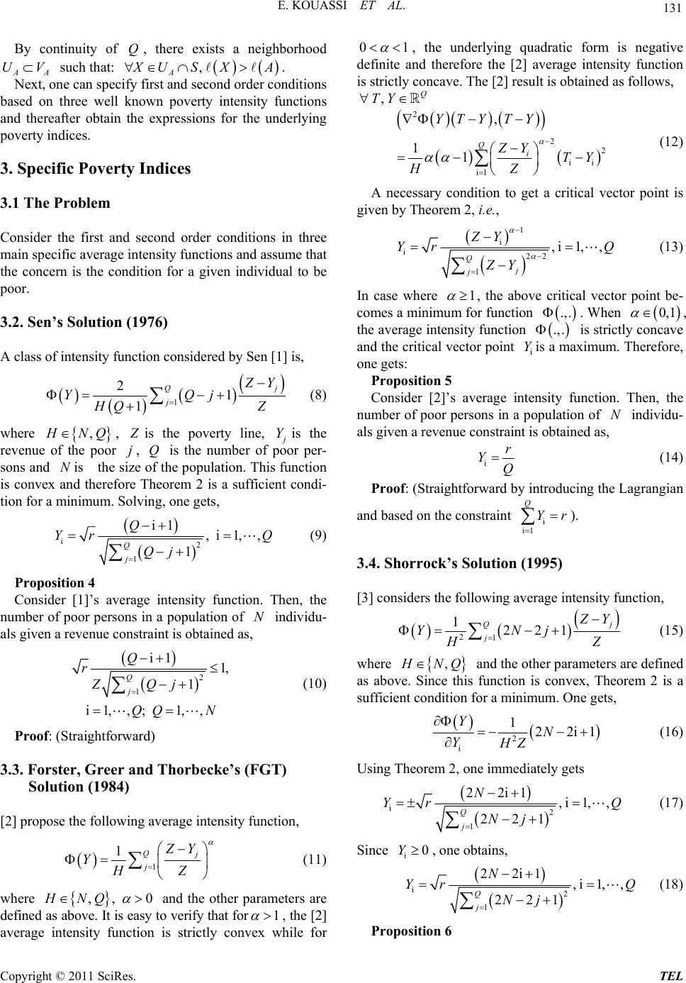

E. KOUASSI ET AL. 131
By continuity of , there exists a neighborhood
such that: Q
AA
UV
 
,
A
X
USX A .
ecify first and second order coNext, one can spnditions
ba
and therthe expressions for the unrlying
po
.1 The Problem
onsider the first and second order conditions in three
intensity functions and assume that
e concern is the condition for a given individual to be
class of intensity function considered by Sen [1] is,
sed on three well known poverty intensity functions
eafter obtain de
verty indices.
3. Specific Poverty Indices
3
C
main specific average
th
poor.
3.2. Sen’s Solution (1976)
A
  

1
1
21
j
Q
j
Z
Y
YQj

 
 (8)
where
HQ Z



,
H
NQ,
Z
is the poverty line,
j
Y
poor
This fun
is the
revenu is the number of
sons and e population. ction
ex and therefore t
o g
e of the poor
Nis th j, e size of th
Q per-
is convTheorem 2 is a sufficiencondi-
tion for a minimum. Slvin, one gets,


i2
1
i1 ,i 1,,
1
Q
j
Q
Yr Q
Qj





 (9)
Proposition 4
Consider [1]’s average intensity function. Th
number of poor persons in a population of individu-
al e constraint is obtained as,
en, the
N
s given a revenu


2
1
i1 1,
1
Q
j
Q
rZQj

 


i1
,,; 1,,QQ N
(10)
Proof: (Straightforwa r d)
3.3. Forster, Greer and Thorbecke’s (FGT)
,
Solution (1984)
[2] propose the fo llowing average intensity fu nction

1j
HZ
1Qj
ZY
Y






 (11)
where and the other parameters are
defi to verify th

,, 0HNQ  
ned as above. It is easy at for1

, the [2]
average intensity function is strictly convex while for
10


 quadratic form is negative
definite and therefore the [2] average intensity function
is strictly concave. The [2] result is obtained as fo llows,
Q
, the underlying
,TY








 
2
2
,
Q
YTY TY
 
  
(12)
2
ii
i1
11i ZY TY
HZ




 



ecessary condition to get a critical v
heorem 2, i.e.,
A n
given by Tector point is


1
j
Y
 
re
i
i22
1
,i 1,,
Q
j
ZY
Yr Q
Z
 





 (13)
In case whe1


um f o r
, the above critical vect
ni m func t io n . When
or point be-
co mes a mi

.,.


0,1  ,
ncave the aver
als
age intnsity function is strictly co
te
poor persons in a population of individu-
e constraint is obtained as,
e

.,.
and the critical vector point i Yis a ma xi mu m. T he refo re ,
one gets:
Proposition 5
Consider [2]’s average innsity function. Then, the
number ofN
given a revenu
ir
YQ

(14)
Proof: (Straightforward by introdu cing the Lagr angian
the constraint
(1995)
ers the following average intensity function,
and based on
[3] consid
i
i1
QYr
).
3.4. Shorrock’s Solution
 

21
1221
j
Q
Z
j
Y
YNj
Z
H


 
 (15)
where


,
H
NQ
. Sincand the other parameters are defined e this function is convex, Theo
condition for a minimum. One gets,
as above
sufficient rem 2 is a


2
i
122i1
YN
YHZ



 (16)
Using Theorem 2, one immediately gets



i2
1221
Q
jNj 

22i1 ,i 1,, N
Yr Q
  (17)
, one obtains,

Since i Y0



i2
22i1 ,i 1,,
21
N
Yr Q
j



 (18)
Proposition 6
12
Q
jN 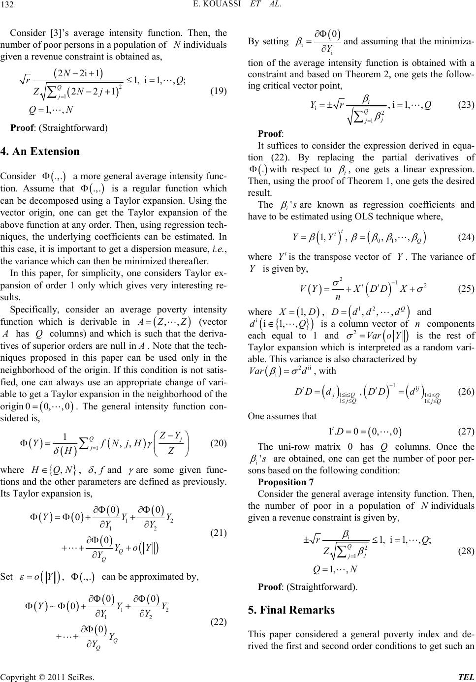


E. KOUASSI ET AL.
132
Consider [3]’s average intensity function. Th
number of poor persons in a population of nd
given a revenue constraint is obtained as,
en, the
ividuals Ni


2
1
1, i1,, ;
221
1, ,
Q
j
rQ
ZN
j
QN







(19)
2N2i1
Proof: (Straightforwa r d)
4. An Extension
Cneral average intensity func-
tio is a regular function which
Taylor expansion. Using the
et the Taylor expansion of the
tion atg co
onsider

.,. a more ge
. Assume that

.,. n
can be decomposed usi
ector origin, one can g
ng a
v
above func any order. Then, using regression tech-
niques, the underlyinefficients can be estimated. In
this case, it is important to get a dispersion measure, i.e.,
the variance which can then be minimized thereafter.
In this paper, for simplicity, one considers Taylor ex-
pansion of order 1 only which gives very interesting re-
sults.
Specifically, consider an average poverty intensity
function which is derivable in

,,
A
ZZ (vector
A
has Q columns) and which is such that the deriva-
tives of superior orders are null in
A
. Note that the tech-
niques proposed in this paper can be used only in the
neighborhood of the origin. If thisot satis-
fd, one can always use an appropriate change of vari-
able to get a Taylor expansion in thghborhood of the
origin

00,,0. The general intensity function con-
sidered is,
 
condition is n
e nei
ie

1
1,, Q
j
j
Z
Y
YfNjH
HZ





 

 (20)
where

,
H
QN , ,
f

and

are some given func-
tions anedefined as previously.
Its Taylor expansion is,
d the other parametrs are
  


00
0
Q
Q
Y
YoY
Y
 
 



Set
12
12
0
YY
YY



(21)

oY  ,


.,. can be app roxima ted by,
  

12
12
00
~0
0Y



ii
0
Y



Q
Q
YYY
YY
Y
 
 




(22)
By setting and assuming that the minimiza-
tion of the average intensity function is o
constraint and based on Theorem 2, one gets the follow-
ing critical vector point,
btained with a
i2
1
,i 1,,
i
Q
j
j
Q


 (23)
Proof:
It suffices to consider the expression derived in equa-
tion (22). By replacing
Yr

 
the partial derivatives of


.with respect to i

, one gets a linear
using the proof heorem 1, one gets the desired
re
expression.
Then, of T
sult.
The '
i
s

are known as regression coefficients and
have to be estimated using OLS technique where,


01
1,,,,
tQ
YY,
t

 (24)
where t
Y
ven
is the transpose vector of . The variance of
Y Y is giby,


212tt
VYXDDX

n




(25)
where


1,
X
D,


12
,,,
Q
Ddd d and




ii1,dQ is a column vector of n components
ch equal to
,1
ea and

2VaroY
  is the rest of
which
able. This variance is also characterized by
Taylor expansion is interpreted as a random vari-


2ii
d  
i
Var 
 
1
1i 1ii11
,t
QQj
, with
jit
jQ
j
Q
dDD d

 

 (26)
One assumes that

00, ,0
t 
DD 
1.D (27)
The uni-row matrixlumns. Once the 0 has Q co
i'
s

sons bare obtained, one n getnumber of p ased on the follow condn:
Consider the general average intens
tha at
gi
ca
ing the itio oor per-
Proposition 7 ity function. Then,
e number of poor in populion of Nindividuals
ven a revenue constraint is given by,
i1, i1r


2,,;
QQ
5. Final Remarks
This paper considered a general poverty index and de-
rived the first and second order conditions to get such an
1
1, ,
j
j
Z
QN





(28)
Proof: (Straightforwa r d).

E. KOUASSI ET AL.
133
in] indices based on specific
innsity functions are then obtained as special cases of
ty index. An extension based o
rge class of intensity function is also investigated.
12718
dex. The well known [1,3
te
this more general povern a
la
6. References
[1] A. K. Sen, “Poverty: An Ordinal Approach to Measure-
ment,” Econometrica, Vol. 44, No. 2, 1976, pp. 219-231.
doi:10.2307/19
] J. Foster, J. Greer and E. Thorbecke, “A Class of De-[2 composable Poverty Measures,” Econometrica, Vol. 52,
No. 3, 1994, pp. 761-765. doi:10.2307/1913475
[3] A. F. Shorrocks, “Revisiting the Sen Poverty Index,”
Econometrica, Vol. 63, No. 5, 1995, pp. 1225-1230.
doi:10.2307/2171728