Theoretical Economics Letters, 2011, 1, 118-121
doi:10.4236/tel.[phone] Published Online November 2011 (http://www.SciRP.org/journal/tel)
Durability and Economic Dynamics
Atsuo Utaka*
Kyoto University Yoshida-hommachi, Sakyo-ku, Kyoto, Japan
Received August 25, 2011; revised October 3, 2011; accepted October 10, 2011
Abstract
This paper investigates how product’s durability affects the dynamic properties of the economy, using a sim-
ple overlapping generations model with durable goods. One of the chief characteristics of the durable-goods
market is that a sale condition at a certain period affects another period’s condition. It is shown that this in-
teraction causes oscillatory equilibria that diverge from the stationary point. Hicks [1] argued that unstable
oscillations in the economy lead to endogenous business cycles. This paper’s result provides one reason of
how unstable oscillations occur from firm’s optimizing behavior.
Keywords: Oscillatory Equilibria, Durability
1. Introduction
This paper investigates how product’s durability affects
the dynamic properties by using a simple overlapping
generations model with a durable-goods monopolist. In
the real economy, the market trends of durable goods
have a large effect on business cycles. One of the chief
characteristics of the durable-goods market is that busi-
ness conditions at a certain period affect future condi-
tions, which can cause economic fluctuations.
Benhabib and Day [2], Grandmont [3], Farmer [4],
and Reichlin [5] analyzed the existence of endogenous
cycles in overlapping generations models. Their models
are based on the general equilibrium model, and do not
consider durable goods. On the other hand, Conlisk et al.
[6] and Sobel [7] constructed the durable-goods mo-
nopolist model, in which new consumers enter at every
period, investigated the dynamics of the durable-goods
market.1 They mainly inv estigated the pricing (and sales)
strategy that the monopolist uses, as well as its commit-
ment problem. In contrast, this paper focuses on a dif-
ference equation concerning the dynamical system of the
durable-goods market.
It is assumed that the firm can increase the demand of
its product with its marketing strategy. If the firm strives
to sell as many products as possible in a certain period,
the demand for its products will decline in the following
periods. To maximize its total p rofits over the long term,
the durable-goods producer takes these dynamic interac-
tions into consideration, which affects the dynamic pro-
perties of the economy. Consequently, it is shown that
there occur oscillatory equilibria that diverge from the
stationary point. Hicks [1] considered a simple dynamic
model based on “acceleration principle”, and argued that
in cases where the dynamic system has unstable oscilla-
tions, endogenous business cycles occur because of a
ceiling caused by full employment and a floor by in-
vestment. (For more detailed analyses concerning Hicks’
trade cycle model, see Hommes [8,9], Saura et al. [10],
Puu [11], and Matsumoto and Szidarovszky [12].) This
paper’s analysis provides one way of explaining the
Hicks’ trade cycle from the viewpoint of firm’s optimiz-
ing behavi or.
2. The Model
I construct a simple overlapping generations model.
There exists a durable-goods monopolist and consumers.
The monopolist firm infinitely continues. On the other
hand, consumers live two periods. They use either zero
or one unit of the durable-goods in each period. Let us
define consumers who enter the market at period t as
generation t consumers. Namely, in period t, there exist
generation t-1 consumers in their second stage and gen-
eration t consumers in their first stage. The population of
each generation is n.
*I would like to thank an anonymous referee for helpful comments.
1It is known that interaction between decisions at different periods
causes various kinds of time-inconsistency problem. For the survey o
f
durable-goods analyses, see Waldman [13].
It is possible for the product to break down. In other
words, the durable goods last two periods (only one pe-

119 A. UTAKA
riod) with probability


1


.2 The benefits each con-
sumer obtains by using the durable-goods is i in his
i-th stage (i = 1, 2). Without loss of generality, the pro-
duction cost of the durable-goods is assumed to be zero.
The discount factor of both consumers and the producer
is
u

, and they are risk neutral. The secondhand market
does not exist .
It is assumed that the demand of the durable-goods can
be increased by the firm’s marketing strategy. Let us
suppose informative advertising as the marketing strat-
egy. Then, the higher the marketing (advertising) level
becomes, the more consumers recognize the existence of
the product. Accordingly, the probability that the infor-
mation on the product reaches each consumer is assumed
to be

t

f
M, where t
M
stands for marketing expen-
diture by the firm. Consumers who recognize the exis-
tence of the products decide whether to buy them at the
price the monopolist offers.
The shape of

t

f
M is as follows.
Assumption 1
 
'0, ''
tt
fM fM0 and for all

1
t
fM t
M
,
and

'0f
In addition, it is assumed that
Assumption 2

11
2
1
2
t
uu
u
fM 1

 


 
t


for any ()
1t
M1, 2,,t
Under this assumption, we obtain the following result.
Lemma
The monopolist in any period t decides to set a price
2 on the products, and sells the products to con-
sumers belonging to generations t and t-1 (those who did
not buy them in period t-1 and whose goods were broken
down).
pu
Proof
[See appendix for the detail.]
In other words, the price of the product becomes con-
stant through all periods. Then, the total demand in pe-
riod t becomes
  
1
1tt nfMfMfM 



.
2.1. Marketing De cision
From now on, let us analyze the monopolist’s behavior
on the marketing strategy.
First, I analyze the case where 0


2u, namely, the products are non-durable-goods. If 21 , it is opti-
mal for the monopolist in each period to sell the products
to both generations. Then, the monopolist’s problem at
any period t is
u

2
2
ttt
M
M
axnuf MM


The first order condition of this problem becomes


2
2' 1
t
nu fM0


Then, the marketing (and production) level is constant
through all periods. Naturally, oscillatory equilibria never
exist.
Next, let us investigate the monopolist’s profit-maxi-
mizing problem. As shown before, since the price of a
product becomes constantly 2, the remaining decision
by the monopolist is about the marketing level. The
problem of the monopolist at period t becomes (see (1a)).
u
The first order condition of this problem becomes (see
(1b)).
In other words, the dynamical system is described by
the second order difference equation. Given initial values
0
M
and 1
M
, the equilibrium trajectories of this sys-
tem are determined by (1b).
2.2. Stationary Equilibrium
Stationary equilibrium is derived from the following
equation.






**
2'21nufMf M
 1

  (2)
Let us assume that

 


2'0 201nu ff


 .
Then, we obtain the following result.
Theorem 1
There exists a stationary equilibrium.
Proof
Let us define the function




2'21nufMf M
 
as


A
M. Under assumption 1,
  
121
, ,...,0
1
tt
jtjtjtj tj
MMMj
Maxnuf MfMfMM 






 


(1a)
      
21 11
2
1
'2' 101 2
'
tt tttt
t
nufMfMf MfMfMfM
nu fM
 


 

.
(1b)
2In this m odel, repair market is not considered.

A. UTAKA
120
 












2
2
'''21 1'AMnufMfMf M  

 

0.
1
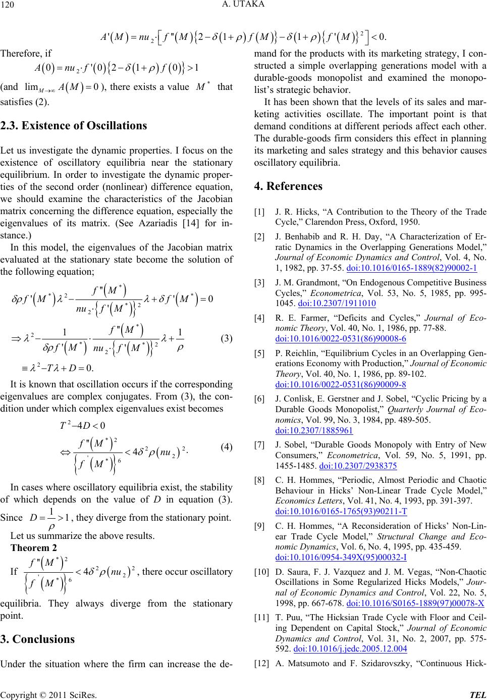
Therefore, if
  
2
0'0210Anuf f   
(and ), there exists a value

lim 0
MAM  *
M
that
satisfies (2).
2.3. Existence of Oscillations
Let us investigate the dynamic properties. I focus on the
existence of oscillatory equilibria near the stationary
equilibrium. In order to investigate the dynamic proper-
ties of the second order (nonlinear) difference equation,
we should examine the characteristics of the Jacobian
matrix concerning the difference equation, especially the
eigenvalues of its matrix. (See Azariadis [14] for in-
stance.)
In this model, the eigenvalues of the Jacobian matrix
evaluated at the stationary state become the solution of
the following equation;
 
 

 


*
*2 *
*2
2
*
2
**2
2
2
''
'
'
''
1
''
0.
fM
fM fM
nuf M
fM
fM nuf M
TD
 





 


'
0
1


(3)
It is known that oscillation occurs if the corresponding
eigenvalues are complex conjugates. From (3), the con-
dition under which complex eigenvalues exist becomes




2
*2
2
2
'*6
40
'' 4
TD
fM nu
fM



2

(4)
In cases where oscillatory equilibria exist, the stability
of which depends on the value of D in equation (3).
Since 11D

, they diverge from the stationary point.
Let us summarize the above results.
Theorem 2
If




*2
2
2
'*6
'' 4 fM nu
fM
 2 , there occur oscillatory
equilibria. They always diverge from the stationary
point.
3. Conclusions
Under the situation where the firm can increase the de-
mand for the products with its marketing strategy, I con-
structed a simple overlapping generations model with a
durable-goods monopolist and examined the monopo-
list’s strategic behavior.
It has been shown that the levels of its sales and mar-
keting activities oscillate. The important point is that
demand conditions at different periods affect each other.
The durable-goods firm considers this effect in planning
its marketing and sales strategy and this behavior causes
oscillatory equilibria.
4. References
[1] J. R. Hicks, “A Contribution to the Theory of the Trade
Cycle,” Clarendon Press, Oxford, 1950.
[2] J. Benhabib and R. H. Day, “A Characterization of Er-
ratic Dynamics in the Overlapping Generations Model,”
Journal of Economic Dynamics and Control, Vol. 4, No.
1, 1982, pp. 37-55. doi:10.1016/0165-1889(82)90002-1
[3] J. M. Grandmont, “On Endogenous Competitive Business
Cycles,” Econometrica, Vol. 53, No. 5, 1985, pp. 995-
1045. doi:10.2307/1911010
[4] R. E. Farmer, “Deficits and Cycles,” Journal of Eco-
nomic Theory, Vol. 40, No. 1, 1986, pp. 77-88.
doi:10.1016/0022-0531(86)90008-6
[5] P. Reichlin, “Equilibrium Cycles in an Overlapping Gen-
erations Economy with Production,” Journal of Economic
Theory, Vol. 40, No. 1, 1986, pp. 89-102.
doi:10.1016/0022-0531(86)90009-8
[6] J. Conlisk, E. Gerstner and J. Sobel, “Cyclic Pricing by a
Durable Goods Monopolist,” Quarterly Journal of Eco-
nomics, Vol. 99, No. 3, 1984, pp. 489-505.
doi:10.2307/1885961
[7] J. Sobel, “Durable Goods Monopoly with Entry of New
Consumers,” Econometrica, Vol. 59, No. 5, 1991, pp.
1455-1485. doi:10.2307/2938375
[8] C. H. Hommes, “Periodic, Almost Periodic and Chaotic
Behaviour in Hicks’ Non-Linear Trade Cycle Model,”
Economics Letters, Vol. 41, No. 4, 1993, pp. 391-397.
doi:10.1016/0165-1765(93)90211-T
[9] C. H. Hommes, “A Reconsideration of Hicks’ Non-Lin-
ear Trade Cycle Model,” Structural Change and Eco-
nomic Dynamics, Vol. 6, No. 4, 1995, pp. 435-459.
doi:10.1016/0954-349X(95)00032-I
[10] D. Saura, F. J. Vazquez and J. M. Vegas, “Non-Chaotic
Oscillations in Some Regularized Hicks Models,” Jour-
nal of Economic Dynamics and Control, Vol. 22, No. 5,
1998, pp. 667-678. doi:10.1016/S0165-1889(97)00078-X
[11] T. Puu, “The Hicksian Trade Cycle with Floor and Ceil-
ing Dependent on Capital Stock,” Journal of Economic
Dynamics and Control, Vol. 31, No. 2, 2007, pp. 575-
592. doi:10.1016/j.jedc.2005.12.004
[12] A. Matsumoto and F. Szidarovszky, “Continuous Hick-

121 A. UTAKA
sian Trade Cycle Model with Consumption and Invest-
ment Time Delays,” Journal of Economic Behavior and
Organization, Vol. 75, No. 1, 2010, pp. 95-114.
doi:10.1016/j.jebo.2010.03.010
[13] M. Waldman, “Durable Goods Theory for Real World
Markets,” Journal of Economic Perspectives, Vol. 17, No.
1, 2003, pp. 131-154. doi:10.1257/089533003321164985
[14] C. Azariadis, “Intertemporal Macroeconomics,” Black-
well, New York, 1993.
Appendix
Here, I analyze the price of the durable goods. In any
period t, the monopolist has two options; to sell the
products to both generations t-1 and t consumers, or to
sell them only to generation t consumers at a higher
price.
In the former case, the price of a product should be
2. It is because generation t-1 consumers use the
products only during one period, if they buy the product
at period t. If we describe marketing expenditure in this
case as
pu
a
M
, total demand in period t becomes



 
1
1aa
tt
nfMfMfM 





a
t


.
Therefore, profits of the monopolist in period t are
 


1
22aa
tt
nufMfM M 


a
t
(A1)
In the latter case where the monopolist sells the prod-
ucts only to generation t consumers, the price becomes
12
pu u



. (At this price, Generation t-1 does not
buy the products under assumption 2.) Let us denote
marketing expenditure in this cs yt M. Since the
demand in periodase a t is


yt
M, profits of the monopo-
list in period t becnf me o



12
y
y
t
nuuf MM   
t
(A2)
Under assumption 2, for all ,
1t
M



1
21
11
2
2
2.
t
t
u
ufM
ufMu

2
u





 
Then, it can be easily shown that profits (A1) become
larger than (A2) at their maximum levels of and
. Consequently, it is optimal for the monopolist in
period t to sell their products to both generations t-1 and t
consumers.
at
M
yt
M