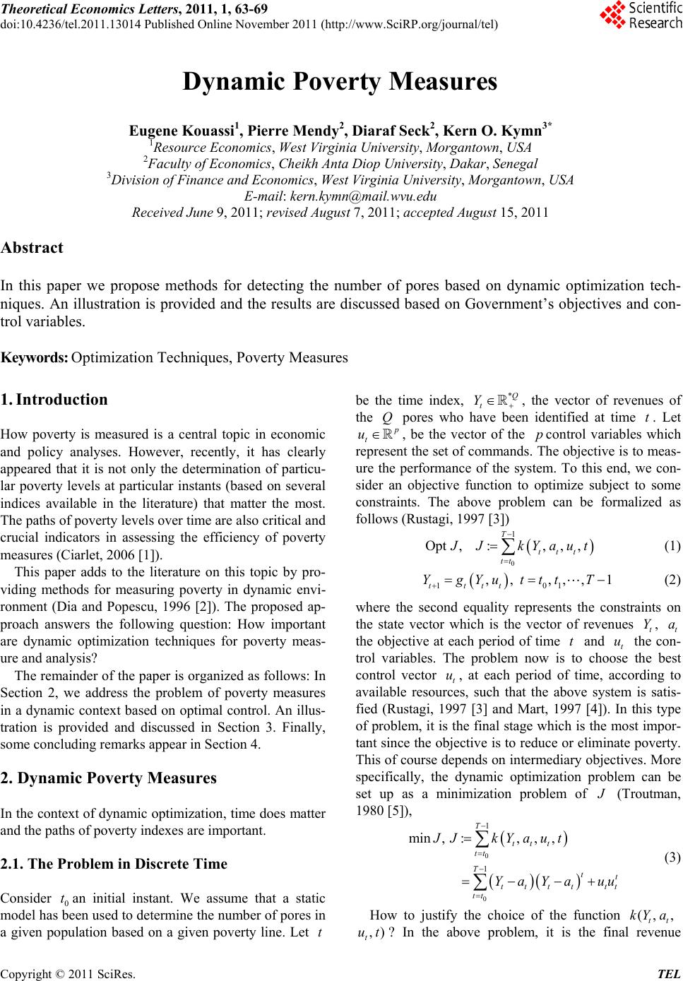Theoretical Economics Letters, 2011, 1, 63-69
doi:10.4236/tel.[phone] Published Online November 2011 (http://www.SciRP.org/journal/tel)
Dynamic Poverty Measures
Eugene Kouassi1, Pierre Mendy2, Diaraf Seck2, Kern O. Kymn3*
1Resource Economics, West Virginia University, Morgantown, USA
2Faculty of Economics, Cheikh Anta Diop University, Dakar, Senegal
3Division of Finance a nd Eco nomi c s, West Virginia University, Morgantown, USA
Received June 9, 2011; revised August 7, 2011; accepted August 15, 2011
Abstract
In this paper we propose methods for detecting the number of pores based on dynamic optimization tech-
niques. An illustration is provided and the results are discussed based on Government’s objectives and con-
trol variables.
Keywords: Optimization Techniques, Poverty Measures
1. Introduction
How poverty is measured is a central topic in economic
and policy analyses. However, recently, it has clearly
appeared that it is not only the determination of particu-
lar poverty levels at particular instants (based on several
indices available in the literature) that matter the most.
The paths of poverty levels over time are also critical and
crucial indicators in assessing the efficiency of poverty
measures (Ciarlet, 2006 [1]).
This paper adds to the literature on this topic by pro-
viding methods for measuring poverty in dynamic envi-
ronment (Dia and Popescu, 1996 [2]). The proposed ap-
proach answers the following question: How important
are dynamic optimization techniques for poverty meas-
ure and analysis?
The remainder of the paper is organized as follows: In
Section 2, we address the problem of poverty measures
in a dynamic context based on optimal control. An illus-
tration is provided and discussed in Section 3. Finally,
some concluding remarks appear in Section 4.
2. Dynamic Poverty Measures
In the context of dynamic optimization, time does matter
and the paths of poverty indexes are important.
2.1. The Problem in Discrete Time
Consider 0an initial instant. We assume that a static
model has been used to determine the number of pores in
a given population based on a given poverty line. Let
be the time index,
t
t
*Q
t
Y

, the vector of revenues of
the pores who have been identified at time . Let Qt
p
t, be the vector of the control variables which
represent the set of commands. The objective is to meas-
ure the performance of the system. To this end, we con-
sider an objective function to optimize subject to some
constraints. The above problem can be formalized as
follows (Rustagi, 199 7 [3] )
up
,

Opt ,,,
ttt
0
1
:T
tt

J
Jk


Yaut (1)


1
,,
tt
Yu 01 ,,,
tt
Yg ttT
t1 (2)


where the second equality represents the constraints on
the state vector which is the vector of revenues t, t
the objective at each period of time and t the con-
trol variables. The problem now is to choose the best
control vector t, at each period of time, according to
available resources, such that the above system is satis-
fied (Rustagi, 1997 [3] and Mart, 1997 [4]). In this type
of problem, it is the final stage which is the most impor-
tant since the objective is to reduce or eliminate poverty.
This of course depends on intermediary objectives. More
specifically, the dynamic optimization problem can be
set up as a minimization problem of
Y a
t u
u
J
(Troutman,
1980 [5]),


min ,:,
t
tt
tt tt
JJ t
Ya uu

,
tt
au
0
0
1
1
,
T
tt
T
tt
tt
kY
Ya








(3)
How to justify the choice of the function
? In the above problem, it is the final revenue
(,kY ,
tt
a
,
t
ut)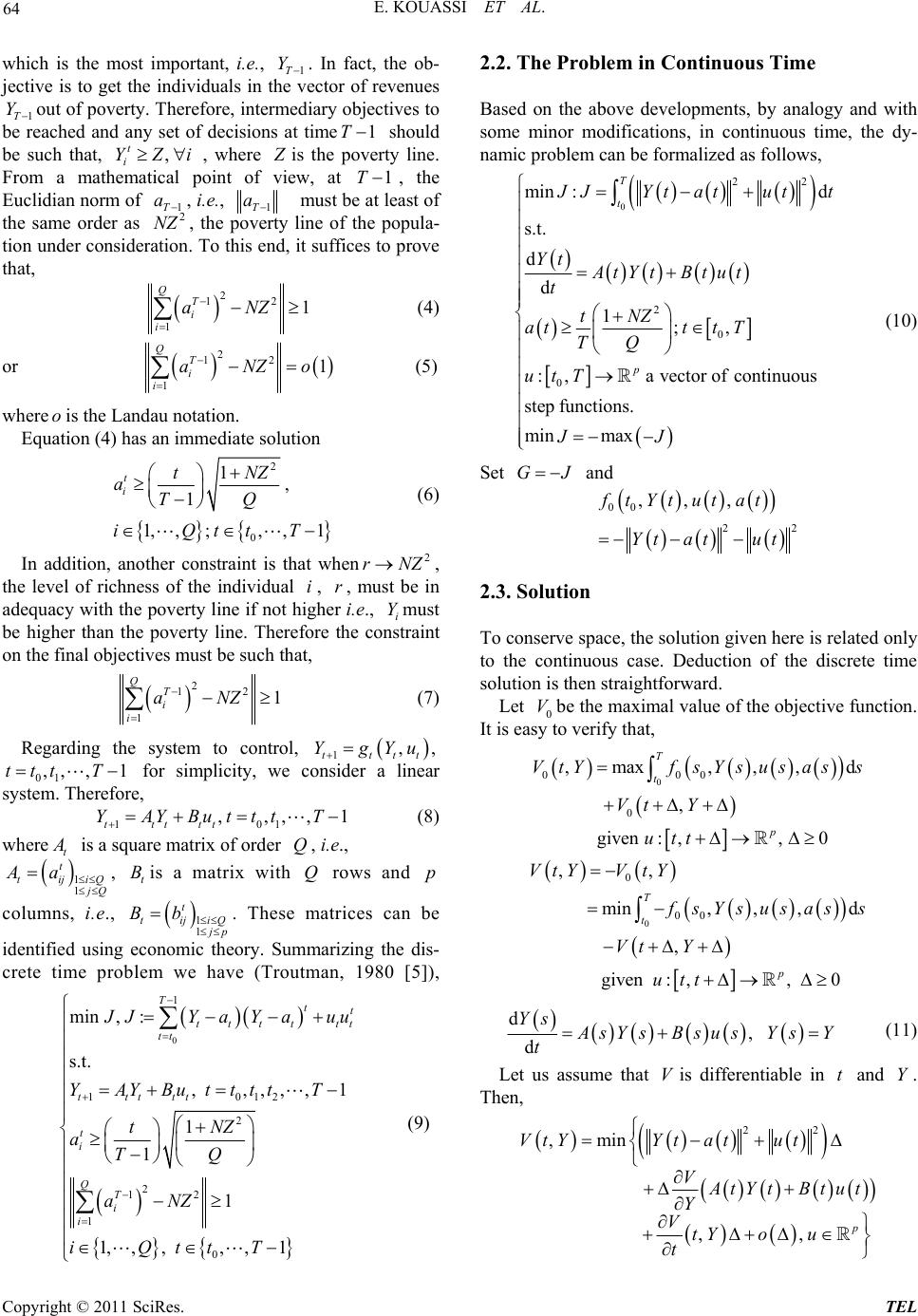

E. KOUASSI ET AL.
64
which is the most important, i.e., 1T. In fact, the ob-
jective is to get the individuals in the vector of revenues
1Tout of poverty. Therefore, intermediary objectives to
be reached and any set of decisions at time should
be such that, , where
Y
Y1T
,
t
i
YZi
Z
is the poverty line.
From a mathematical point of view, at 1T

, the
Euclidian norm of , i.e.,
1T
a1
T must be at least of
the same order as , the poverty line of the popula-
tion under consideration. To this end, it suffices to prove
that,
a
2
NZ

2
12
1aNZ

1
Q
i
i
T


 (4)
or


o
2
12
1aNZ

1
QT
i
i
 (5)
whereois the Landau notation.
Equation (4) has an immediate solution

1
1, ,iQ



2
0
1,
;, ,1
t
itNZ
aTQ
ttT





r
r
(6)
In addition, another constraint is that when,
the level of richness of the individual , , must be in
adequacy with the poverty line if not higher i.e., imust
be higher than the poverty line. Therefore the constraint
on the final objectives must be such that,
2
NZ
iY
2
T
i12
1
1
Q
i
aNZ


 (7)
Regarding the system to control,


,,Yu
1tt

1
1T
tt
Yg
01 for simplicity, we consider a linear
system. Therefore,
,, ,1t Ttt
1ttt
Y 0 ,,,,
tt
YAButtt
 (8)
where t
A
is a square matrix of order , i.e., Q

1
1iQtij
t
j
Q
Aa


, is a matrix with Q rows and
columns, i.e.,
t
B p

t
ti1
1iQ
j
j
p


Bb. These matrices can be
identified using economic theory. Summarizing the dis-
crete time problem we have (Troutman, 1980 [5]),



0
1
2
12
1
1
,
T
tt
t

10
1
2
1
0
min ,:
s.t.
,,,,,
1
1, ,, ,1
t
tttt
tttt
t
i
QT
i
i
2
1
t
tt
J
JY
YB
aN







aYa
YA utttt
tNZ
aTQ
Z
iQttT






















uu
T


(9)
2.2. The Problem in Continuous Time
Based on the above developments, by analogy and with
some minor modifications, in continuous time, the dy-
namic problem can be formalized as follows,
 


  
 


0
22
2
0
0
min :d
s.t.
d
d
1;,
:,avector ofcontinuous
step functions.
min max
T
t
p
J
JYtatut
Yt AtYt Btut
t
tNZ
atttT
TQ
utT
JJ
t












 




 




(10)
Set GJ

 and




 
00
22
,,,ftYtutat
Yt atut 
2.3. Solution
To conserve space, the solution given here is related only
to the continuous case. Deduction of the discrete time
solution is then straightforward.
Let 0be the maximal value of the objective fun ction.
It is easy to verify that,
V
   


0
000
0
,max,,, d
,
given: ,,0
T
t
p
VtYfsYsusas s
Vt Y
utt


 






   


0
0
00
,,
min,, ,d
,
given: ,,0
T
t
p
VtYV tY
f
sYsus ass
Vt Y
utt



 



 
d,
d
Ys
A
sY sBsusYsY
t


(11)
Let us assume that is differentiable in and Y.
Then, Vt
  


  
 
22
,min
,,p
VtYYtatut
V
A
tYt Btut
Y
VtYo u
t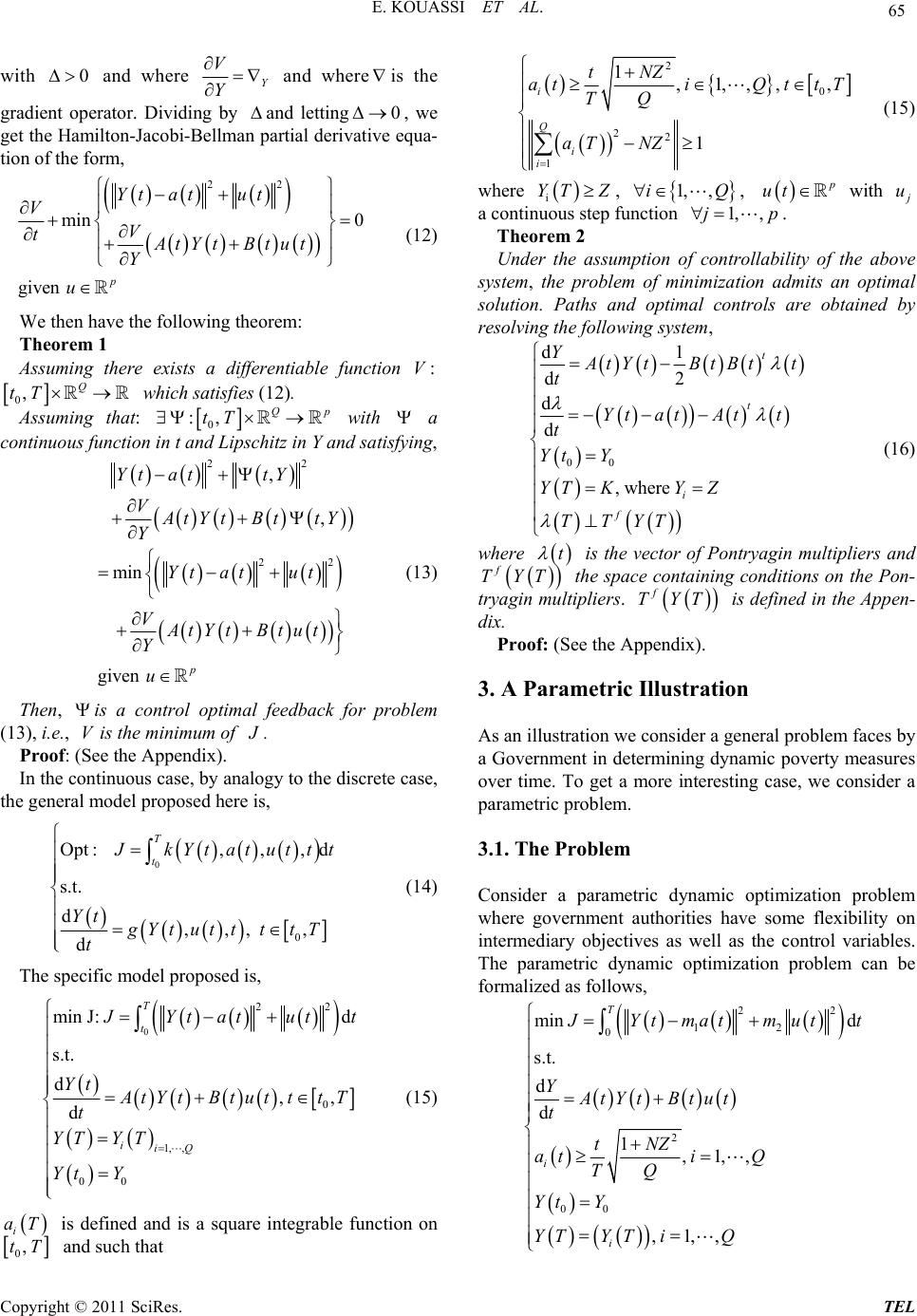




 








65 E. KOUASSI ET AL.
with and where 0 Y
V
Y



 and where

is the
gradient operator. Dividing by and letting, we
get the Hamilton-Jacobi-Bellman partial derivative equa-
tion of the form,
0
 

 

22
min 0
given p
Yt atut
VV
tAtYt Btut
Y
u
















(12)
We then have the following theorem:
Theorem 1
Assuming there exists a differentiable function :V


0,Q
tT which satisfies (12).
Assuming that:


0
:, Q tT 
p
with

a
continuous function in t and Lipschitz in Y and satisfying,
 
  
 

  
22
22
,
,
min
given p
Yt attY
V

A
tYt BttY
Y
Yt atut
VAtYtBtut
Y
u













(13)
Then, is a control optimal feedback for problem
(13), i.e., is the minimum of

V
J
.
Proof: (See the Appendix).
In the continuous case, by analogy to the discrete case,
the general model proposed here is,
   
  


0
0
Opt :,,,d
s.t.
d,,,,
d
T
t
J
kYt at ut t t
Yt
g
Yt ut tttT
t










(14)
The specific model proposed is,
 

  

 

0
22
0
1, ,
00
min J : d
s.t.
d,,
d
T
t
iiQ
J
Yt atutt
Yt
A
tYtBtutttT
t
YT YT
Yt Y






 









(15)

i
aT

is defined and is a square integrable function on

0,tT and such that
  
 
2
0
22
1
1,1,,,,
1
i
Q
i
i
tNZ
atiQttT
TQ
aT NZ


 






(15)
where


i
YT Z,


1, ,iQ ,

p
ut with
j
u
a continuous step function 1, ,jp

.
Theorem 2
Under the assumption of controllability of the above
system, the problem of minimization admits an optimal
solution. Paths and optimal controls are obtained by
resolving the following system,
 
    


  
00
d1
d2
d
d
,where
t
t
i
f
Y
A
tYtBtBt t
t
Yt atAtt
t
Yt Y
YTKYZ
TTYT






 







(16)
where


t  is the vector of Pontryagin multipliers and




T
f
TY the space containing conditions on the Pon-
tryagin multipliers.




f
TYT is d efined in the Appen-
dix.
Proof: (See the Appendix).
3. A Parametric Illustration
As an illustration we consider a general problem faces by
a Government in determining dynamic poverty measures
over time. To get a more interesting case, we consider a
parametric problem.
3.1. The Problem
Consider a parametric dynamic optimization problem
where government authorities have some flexibility on
intermediary objectives as well as the control variables.
The parametric dynamic optimization problem can be
formalized as follows,
 


 


 

22
12
0
2
00
min d
s.t.
d
d
1,1,,
,1,,
T
i
i
J
Ytmatm utt
YAtYtBtut
t
tNZ
ati Q
TQ
Yt Y
YTYT iQ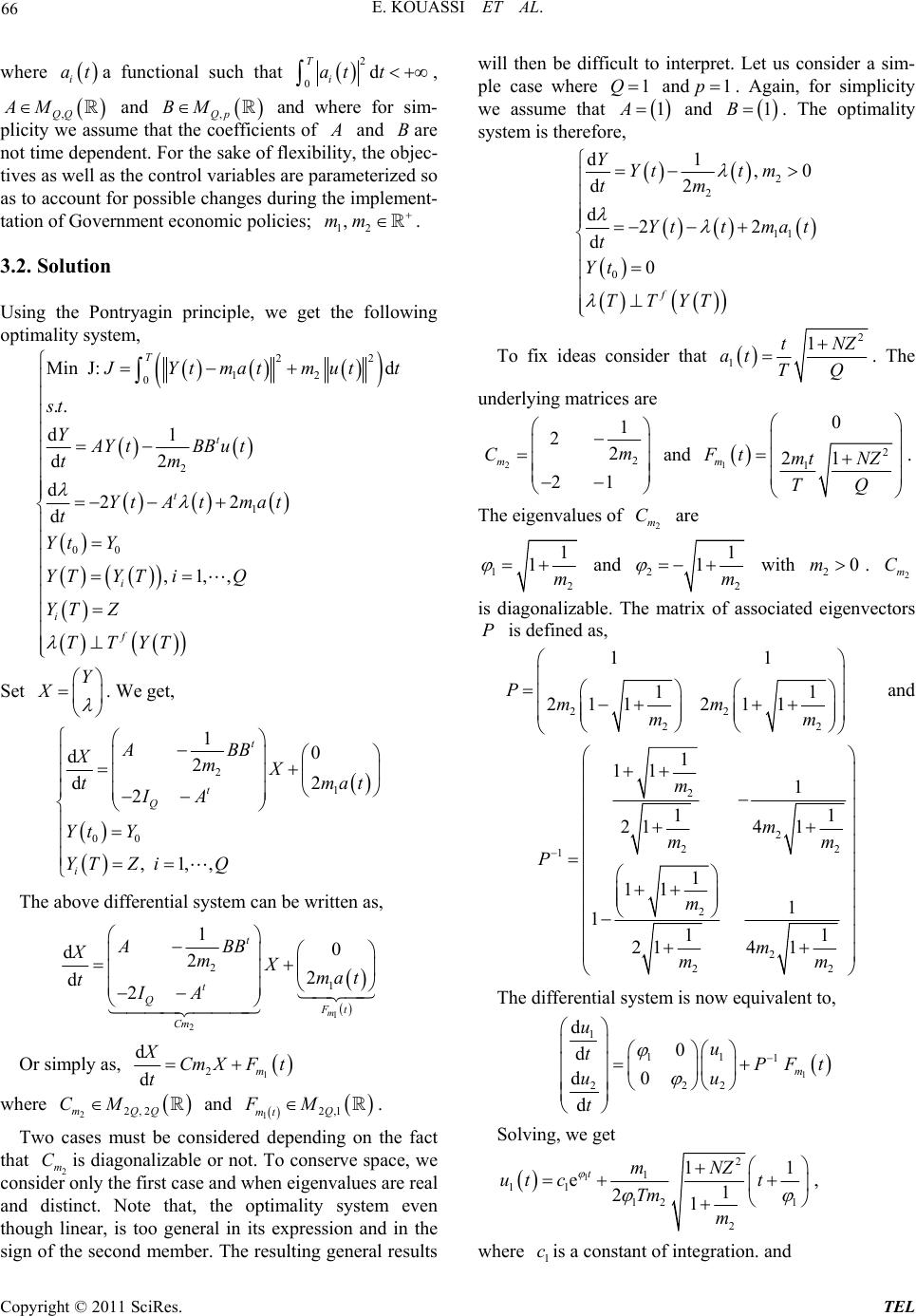



















E. KOUASSI ET AL.
66
where a functional such that

i
at

2
0d
T
i
att


,

,QQ
AM and


,Qp
BM and where for sim-
plicity we assume that the coefficients of
A
and Bare
not time dependent. For the sak e of flexibility, the obje c-
tives as well as the control variables are parameterized so
as to account for possible changes during the implement-
tation of Government economic policies; 12 ,mm

.
3.2. Solution
Using the Pontryagin principle, we get the following
optimality system,
 

 
 

 


 

22
12
0
2
1
00
Min J: d
..
d1
d2
d22
d
,1,,
T
t
t
i
i
f
J
Ytmatm utt
st
YAYtBBut
tm
YtA tmat
t
Yt Y
YTYT iQ
YTZ
TTYT










 












Set Y
X




. We get,



2
1
00
10
d22
d2
,1,,
t
t
Q
i
ABB
XmXma t
tIA
Yt Y
YTZ iQ














The above differential system can be written as,


1
2
2
1
10
d22
d2
m
t
t
QFt
Cm
ABB
XmXma t
tIA










 

Or simply as,

1
2
d
dm
XCmXFt
t
where and .

22,2mQQ
CM


12,1Q
mt
FM
Two cases must be considered depending on the fact
that 2
mis diagonalizable or not. To conserve space, we
consider only the first case and when eigenvalues are real
and distinct. Note that, the optimality system even
though linear, is too general in its expression and in the
sign of the second member. The resulting general results
will then be difficult to interpret. Let us consider a sim-
ple case where
C
1Q

and. Again, for simplicity
we assume that 1p


1A and . The optimality
system is therefore,

1B
 



00
f
Yt
Yt
TT

 
2
22
t m
t m
T



2
11
d1
,0
d2
d
d
Y
tm
at
t
Yt
Y




















To fix ideas consider that 2
1tNZ
TQ

1
at. The
underlying matrices are
22
1
2
1
m





2
2
m
C 

and

12
m
Ft2
1
0
1 mt NZ
TQ






.
The eigenvalues of are
2
m
C
12
1
1m   and
2
1
1m 
2
  with .
is diagonalizable. The matrix of associated eigenvectors
is defined as,
20m2 m
C
P
22
22
11
11
211 211
Pmm
mm


 
 

 






and
2
2
22
1
2
2
22
1
11 1
11
214 1
1
11 1
111
214 1
m
m
mm
P
m
m
mm


















 




The differential system is now equivalent to,

1
1
1 11
2 22
d0
d0
d
d
m
uu
tPFt
uu
t




 

 
 

 


Solving, we get

1
2
1
11 12 1
2
11
e1
21
tmNZ
ut ct
Tm m





 



,
where is a constant of integration. and
1
c

67 E. KOUASSI ET AL.

2
2
1
22 22 2
2
11
e1
21
tmNZ
ut ct
Tm m








2
cbeing a constant of integration as well. Since,
1
UPX
X
PU

where , we obtain,


Yt
Xt







1
22 2
22
11
11
211 211
Yt u
mm
u
tmm



 
 
 

 



 



After a bit of algebra we get,


 
11
11
2
1
12 2
12
2
1
12 2
11 1
ee1
211
ee
211
tt
tt
mt
Yt ccNZ
Tm
mt NZ
cc
tT






 










The optimal controlis given by

ut
 
2
1
2
ut t
m
  .
We now discuss seve ral cases .
3.3. Discussion
Case 1: and .
10m
20m 

1
1
if 0
if 0
c
Yt c
 

 
,

1
1
if 0
if 0
c
tc 
 

 

a nd

1
1
if 0
if 0
c
ut c
 



Poverty can be greatly improved on the condition that
intermediary objectives and control variables be realistic
and comprehensive.
Case 2: and fixed.
10m
2 m

11
12
ee
tt
Yt cc

 
 ,

11
12
11
ee
211
tt
cc
t












and

11
12
211
ee1
11
tt
cc
ut m








Poverty can be gradually improved if intermediary
objectives are reachable and control variables reasonably
selected.
Case 3: and .
10m
2 m

12
ee
tt
Ytcc   ,

2
2
if 0
if 0
c
tc 
 

 

and

2
2e
t
utc  
Poverty can be gradually improved but many control
variables can create entropy in the system.
Case 4: fixed and .
1
m20m 

1
1
if 0
if 0
c
Yt c






,

1
1
if 0
if 0
c
tc 
 



a
nd

1
1
if 0
if 0
c
ut c







Realistic intermediary objectives and well chosen con-
trol variables may result in positive impacts in terms of
poverty alleviation.
Case 5: fixed and fixed.
1
The behaviors of
m2 m


 Yt, and depend on
the specific values assigned to and .

t
1
m


ut
2
m
Case 6: fixed and .
1
m2 m


12
ee
tt
Yt c c

 ,

2
2
if 0
if 0
c
tc 
 

 

a nd

1
1
if 0
if 0
c
ut c







Fixed objectives can be beneficiary for poverty im-
provement but many control variables can negatively
affect the system.
Case 7: and .
1
m 20m 


Yt,


t 
and


ut oscillate to , a case of
uncertainty. 
Case 8: and fixed.
1
m 2 m


Yt,


t   and

ut
Many objectives with reasonable control variables
may result in poverty improvement.
Case 9: and .
1
m 2 m


Yt ,


t  and


utoscillate to, another case
of uncertainty. 
4. Final Remarks
How important are dynamic optimization techniques for
poverty analysis? In dynamic settings, the paths of in-
comes are essential and the paper provides methods ac-
cordingly. It remains to establish optimality and stability
criteria for the characterization of the various paths in a
future research.
5. References
[1] P. G. Ciarlet, “Introduction à l’analyse Numérique Ma-
tricielle et à l’optimisation,” Dunod, Paris, 2006.
[2] J. M. Dia and D. Popescu, “Commande Optimale, Con-
ception Optimisée des Systèmes,” Diderot Arts et Sci-
ences, Paris, 1996.
[3] J. S. Rustagi, “Optimization Techniques in Statistics,” AP
Harcourt Brace and Company Publishers, San Diego, 1997.
[4] R. Mart, “Optimisation Intertemporelles: Application aux

E. KOUASSI ET AL.
68
Modèles Macroéconomiques,” Economica, Paris 1997.
[5] M. Troutman, “Calculus of Variations with Elementary
Convexity,” Springer-Verlag, New York, 1980.
where







 

**
**
,,
,
Y
D tYtVtYt
A
tY tBttY t
 





Appendix: Theorems and Proofs
Theorem 1
Let


0,ttT, and
Q
Y


00
:,
p
utTbe a vec-
tor of functions which represents control variables and

0
Y

the solution to,
We have,
 




 

 





 


**
0
** *
**
0
** *
0,,,
,,
min,,,
,,
Y
Y
VftYt tYt
t
VtYtAtYtBttYt
ftYttYt
VtY tAtY tBttY t





 





 


 
 
.
00
.
00 0
,,
YAYBu
YtYt T

 






.
Let

*
Y

be the solutio n to, given
p
u
 
 
.**
.*00 0
,,
YAYBu
Yt YtT
*

 






Thus,
 




 




 

**
0
**
0
** *
,,,
,,,
,,
Y
ftYttYt
VftYttYt
t
VtYtAtYtBttYt


 



 


where
 

*
,uY

*

  . The assumption on

insures the existence of the solution to the above system.
To show that is an optimal feedback control, we need
to prove that, 
 

 

0
0
22
**
22
*0
d
d
T
t
T
t
Yt atutt
Yt atutt




Hence,





 


0
**
00
**
0
,,
,,,
T
t
VTY TVtYt
d
f
tY ttY tt

 

Set,
 

 
22
** **
0,,
f
tY t utY tatut and On the other hand,
 

 

22
**
00 0
,,ftYtutYt atut
On the one hand,






0
** *
00 d
,,,
d
T
t
V
VTYTVtYttY tt
t

d








*
** *
d
d,, ,
dd
Y
Yt
VV
tYttYt VtYt
tt










 





0
0
0000
0
00
0
,,
d,d
d
,d
,d
d
T
t
T
Y
t
VTY TVtYt
VtY tt
t
VtY tYt
VtY tt
tt















t
We can immediately notice that
p
u,
    


and
  
***
d
d
Yt
A
tYtBtu t
t
where . Since by assumption,
 

*
,uttYt

*


 


    

*
0
0
,,
min, ,
,
Y
ftYt D
ftYtut
VtYtAtYt Btut


 

    

 
 



0
00 0
0
**
0
*
*
d
,,, d
d
min, ,,d
,,,
d
,,given
d
Y
Y
p
Y
Yt
ftYtutVtYt t
Yt
ftYt utVtYtt
ftYt tYt
Yt
VtY tu
t








 
Hence,









0
000
*
00
,,
,, d
T
t
VTY TVtYt
0
f
tY tutt



given
p
u

69 E. KOUASSI ET AL.
We then conclude using the Hamilton-Jacobi-Bellman
equation and the fact that


*000
Yt Yt Y
0
0
d
, that
 

  
00
**
000
,, d,,
TT
tt
f
tYtu ttf tYtu tt

Theorem 2
We have,
 

  

    
0
22
0
1
min :d
s.t.
d,0
d
0
,,
T
t
p
ii
iQ
J
JYtatut
Yt
t
A
tYtBtuttT
t
YY
YtYTYT Zut






 











with a continuous step function, .
The Hamiltonian is,

ut 1, ,jp 
 

 
 
22
00
,,,
t
HtYt utt
pYtatput
tAtYtBtut




 
where is the vector of Pontryagin multipliers. The
first order conditions are,

t 
  
,,, d,1,,
di
i
HtYt uttiQ
Yt
  

 

,,,d,1,,
di
i
HtYt uttYiQ
t




Thus,
 

   
 
0
01
,,,
2
2
i
t
ii i
Q
ii jji
j
HtYt utt
Y
pYt attAtYt
Y
pYt at













where

1,ijQ
ij
A
t 
 . Finally, we get
  

,,,d
d
i
HtYt uttt
Yt
 
. We now have the fol-
lowing differential system,
  

1,
01
d2
dij Q
Q
ii jij
j
tpYt at
t




and
 


0
ff
TY GYt   . In our case,
;


f
d
GIGYt
w
here 0
ff
f
x
Tb
G







,
   
0
ff
TYtYt
G







,
:
f
QQ
G,

00
00
x
Tb
gx











,
 
0000
0TY GY








.
At the optimum, we have

 


0
.,. 2
0,1, ,
t
j
jj
HputBt u t
uu
jp





 
0
20
t
j
putB tt 

.
1) If 00p

, then
  

0
1
2
t
utBtt
p
  .
2) If 00p

, then . By assumption we
have,
 
0
t
Bt t  

 
d
d
Yt
A
tYt Btut
t which is control-
lable on


0, T. Consider

,t

the function of transi-
tion matrices of

 
Ytd
d
A
tYt
t. The assumption of
controllability is equivalent to


,,
00
Qt tB
T


0,

 

.
We claim that if the system is controllable, then 00p

,
otherwise from
    
t
0
d2
d
t
pYtatAt
t

 
we would have deduced,
 


,
t
tTt   T, and
 
0
t
Bt t 

. Thus, .
Hence,

0t  

,0,
t
tTtBtT




 0T0t 

, which is one condition
since and
0
p


t 
0
p cannot both be equal to zero at a time. Therefore, 0

. We can now normalize the
system by setting0 p1

. The path and optimal control
are obtained by solving the following system,

  
    
 

0
d1
d2
d2
d
0, ,,
,1,,
t
t
t
i
Yt
A
tYtBt Btt
t
Yt atAtt
t
YYYtKZZ
YT ZiQ






 







