Int. J. Communications, Network and System Sciences, 2011, 4, 704-708
doi:10.4236/ijcns.2011.411086 Published Online November 2011 (http://www.SciRP.org/journal/ijcns)
Multilayer Hex-Cells: A New Class of Hex-Cell
Interconnection Networks for Massively Parallel Systems
Mohammad Qatawneh
Computer Science Department, University of Jordan, Amman, Jordan
Received September 22, 2011; revised October 13, 2011; accepted November 10, 2011
Abstract
Scalability is an important issue in the design of interconnection networks for massively parallel systems. In
this paper a scalable class of interconnection network of Hex-Cell for massively parallel systems is intro-
duced. It is called Multilayer Hex-Cell (MLH). A node addressing scheme and routing algorithm are also
presented and discussed. An interesting feature of the proposed MLH is that it maintains a constant network
degree regardless of the increase in the network size degree which facilitates modularity in building blocks
of scalable systems. The new addressing node scheme makes the proposed routing algorithm simple and ef-
ficient in terms of that it needs a minimum number of calculations to reach the destination node. Moreover,
the diameter of the proposed MLH is less than Hex-Cell network.
Keywords: Multilayer Hex-Cell, Interconnection Network, Parallel System
1. Introduction
The interconnection network strongly affects the per-
formance of parallel machines. Many interconnection
networks were proposed, from the slow but inexpensive
single bus, to the extremely fast and very expensive
cross-bar network [1-4]. In an interconnection network,
degree related to hardware cost and diameter related to
massage passing time is correlated with each other. In
general, as degree of an interconnection network is in-
creased, diameter is decreased, which can increase
throughput in the interconnection network, however, it
increases hardware cost with the increased number of
links of the processors when parallel system is designed
[2,5-7].
Among the wide variety of interconnection networks
structures proposed for parallel computing systems is
hex-cell which received much attention due to the attrac-
tive properties such as embeddability and simple routing
[8]. However, in an identical hex-cell network the di-
ameter increases with the increase of the network size,
which can decrease throughput of the network. Ideally,
we would like to construct a new network that combines
features such as less communication, efficient routing
and capability of embedding other static topologies. This
gives the motivation to develop a new interconnection
network to meet the demands of highly parallel systems.
In this paper, a new interconnection network called
Multilayer Hex-Cells network (MLH), which requires
less diameter than a comparable size hex-cell network
and with a constant network degree, is proposed. An-
other advantage of the MLH network is that it is hierar-
chical network, which makes it suitable for the connec-
tionist models of computations, which requires a very
large number of processors and its applications are hier-
archical in nature. This paper concentrates on a network
that enjoys the same ease of routing as in the hex-cell
network.
The organization of this paper is as follows. Section 2
describes the definition of Hex-Cell network. Section 3
introduces the proposed Multilayer Hex-Cell network.
Section 4 presents the routing algorithm of MLH and
Section 5 summarizes and concludes the paper.
2. Definition of Hex-Cell Network
A Hex-Cell network [8] with depth d is denoted by HC(d)
and can be constructed by using units of hexagon cells,
each of six nodes. A Hex-Cell network with depth d has
d levels numbered from 1 to d, where, level 1 represents
the innermost level corresponding to one hexagon cell.
Level 2 corresponds to the six hexagon cells surrounding
the hexagon at level 1. Level 3 corresponds to the 12
hexagon cells surrounding the six hexagons at level 2 as

M. QATAWNEH705
d
shown in Figure 1. Each level i has Ni nodes, where Ni
= 6(2i – 1) and the total number of nodes in a Hex-Cell
network HC(d) is N = 6d2. Each node in the HC is identi-
fied by a pair (X.Y), where X denotes the line number in
which the node exists, and Y denotes the location of the
node in the line as in Figure 2. A node with the address
1.1 is the first node that exists at line number 1. 1.2 refers
to the second node that exists at line number 1, and so
on.
3. Multilayer Hex-Cells Interconnection
Network
The Multilayer Hex-Cell (MLH) is a modular intercon-
nection network that consists of layers of identical
Hex-Cell networks connected together in a hierarchical
fashion as shown in Figure 3. The MLH is denoted by
MLH(k,d), where k denotes the layer number, and d de-
notes the depth of the identical Hex-Cell. Each Layer k
has Ni nodes, where Ni = 6d2 and the total number of
nodes in MHL network is 6 kd2.
Lemma 1:
The total number of nodes in a MLH(k,d) with k layers
is:
2
6
MLH
Nk. (1)
Proof:
Using the previous definition of HC(d), it can be eas-
ily seen that the total number of nodes at level 1 as
shown in Figure 1 is N1 = 6 nodes, since there is a single
Figure 1. (a) HC (one level); (b) HC (two levels); (c) HC
(three levels).
Figure 2. Addressing nodes in HC.
Figure 3. MLH (2,2).
hexagon cell with six nodes. Level 2 introduces six
hexagon cells (one at each side of the hexagon at level 1).
It can be seen that level (i + 1) has 12 nodes in addition
to corresponding nodes to those at level i. Therefore, the
total number of nodes at level i is:


61 *12621
i
Ni i


  (2)
The total number of nodes in an identical Hex-Cell
network HC(d) with d levels can be expresses as follows:

162 1
d
hc i
N


i


 (3)
Therefore,
2
1261 691 66Ni dddd

 (4)
The total number of nodes in MLH(k,d) with k layers
can be expresses as follows:
2
6
MLH
Nkd. (5)
3.1. Node Degree
The node degree on an interconnection network is de-
fined as the maximum number of edges (links) that a
node can have in the network. It can be easily seen that
the node degree of an identical Hex-Cell with depth 1 (i.e.
HC(1) is 2 and that for HC(d) is 3, for d > 1. Using the
previous definition of MLH(k,d), it can be easily seen
that the network degree of MLH(1,1) is 3 and that for
MLH(k,d) is 4, for k > 1.The network degree is a desir-
able feature in an interconnection network that the max
number of ports does not grow at the same rate as a func-
tion of the number of nodes in the network. In other
words, a network topology which secures constant net-
work degree is highly desirable. Constant node degree
facilitates modularity in building blocks for scalable sys-
tems. The network degree of MLH(k,d) for k > 1 is con-
stant (4) as the network size increases.

M. QATAWNEH 706
3.2. Diameter
The diameter (D) of a network is the maximum shortest
path between any two nodes. If the source and destina-
tion nodes are located in the same layer (i.e. in the iden-
tical HC(d) the diameter is equal to 4d – 1 [8], but if the
source and destination nodes are located in different lay-
ers in MLH(k,d), the number of k (layer) steps required
to reach the destination node as shown in Case 1 and
Case 2 in the proposed routing algorithm in the section 4.
so the diameter of MLH(k,d) is 4d – 1 + k. Figure 4
shows, that the diameter against network size of the
MLH is less than Hex-Cell network.
4. Proposed Routing Algorithm
In order to explain the following algorithm, we use the
layer and line numbering scheme as follows. Each node
in the MLH is identified by a pair (K.X.Y), where k de-
notes the layer number, X denotes the line number in
which the node exists, and Y denotes the location of the
node in the line as in Figure 5. A node with the address
1.1.1 is the first node that exists at layer 1 and line num-
ber 1. The Node1.1.2 refers to the second node that exists
at layer and 1 and line number 1, and so on.
The proposed addressing node scheme can make the
proposed routing algorithm simple and efficient in term
of the number of operations needed to calculate the next
node, especially when the source and destination nodes
are located in different layers as discussed in the Exam-
ples 1 and 2. The number of calculations is equal to n (n
= the difference between the source and destination layer
numbers).
In the proposed routing algorithm for MLH as shown
in Figure 6, the movement from one node to another
node can be done by using one of the following three
cases:
Figure 4. Diameter against the network size.
Figure 5. Addressing nodes in MLH(2,2).
moveUp(Ks,X s ,Y s , K
d
, X d ,Y d )
if(X
s
≠X
d
)
if(X
s
> depth)
if(X
s
-1 = depth && Y
s
is odd) → moveUp(Ks,Xs-1,Y
s
, K
d
, X
d
Y
d
)
else if (Y
s
is even)
if (Y
s
> Y
d
) → moveUp (Ks,Xs,Y
s-1
, K
d
, X
d
Y
d
)
else → moveUp(Ks,Xs,Y
s+1
, K
d
, X
d
Y
d
)
else → moveUp(Ks,X
s-1
,Y
s+1
, K
d
, X
d
Y
d
)
else if (Y
s
is odd)
if ( Y
s
> Y
d
)→ moveUp (Ks,Xs,Y
s-1
, K
d
, X
d
Y
d
)
else → moveUp(Ks,Xs,Y
s+1
, K
d
, X
d
Y
d
)
else→ moveUp(Ks,X
s-1
,Y
s-1
, K
d
, X
d
Y
d
)
else if (Y
s
≠ Y
d
)→ moveHorizontal(K
s
,X
s
,Y
s
, K
d
, X
d
Y
d
)
else → Destination Reached
moveDown (Ks,X
s ,Y s , K
d
, X d ,Y d )
if(X
s
≠X
d
)
if(X
s
> depth)
if (Y
s
is even) moveDown(K
s
,X
s+1
,Y
s-1
,K
d
,X
d
,Y
d
)
if (Y
s
> Y
d
) → moveDown (Ks,Xs,Y
s-1
, K
d
, X
d
Y
d
)
else → moveDown(Ks,Xs,Y
s+1
, K
d
, X
d
Y
d
)
else if (Y
s
is odd)
if (X
s
< depth) moveDown((K
s
,X
s+1
,Y
s+1
,K
d
,X
d
,Y
d
)
else → moveDown(Ks,Xs
+1
,Y
s
, K
d
, X
d
Y
d
)
else→ (Y
s
> Y
d
) → moveUp(K
s
,X
s
,Y
s-1
,K
d
,X
d
,Y
d
)
else→ moveDown (K
s
,X
s
,Y
s+1
,K
d
,X
d
,Y
d
)
else if (Y
s
≠ Y
d
) → moveHorizontal(K
s
,X
s
,Y
s
,K
d
,X
d
,Y
d
)
else → Destination Reached
moveHorizont al (Ks ,X
s ,Y s , K
d
, X d ,Y d )
if(Y
s
≠ Y
d
)
if(Y
s
> Y
d
) → moveHorizontal(Ks,X s ,Y s-1 , K
d
, X d ,Y d )
else → moveHorizontal(Ks,X
s ,Y s+1 , K
d
, X d ,Y d )
else→Destination Reached.
Figure 6. Routing algorithm for MLH(k,d).
CASE 1: If (Ks = Kd) & (Xs > Xd) then moveUp (Ks, Xs,
Ys, Kd, Xd, Yd)
else if (Ks = Kd) & (Xs < Xd) then moveDown(Ks, Xs, Ys,
Kd, Xd, Yd)
else if ((Ks = Kd) & (Xs = Xd) then moveHorizontal(Ks,
Xs, Ys, Kd, Xd, Yd).
CASE 2: If (Ks > Kd) then (Ks – 1, Xs, Ys, Kd, Xd, Yd).
CASE 3: If (Ks < Kd) then (Ks + 1, Xs, Ys, Kd, Xd, Yd).
where, Ks is the layer number of source node, Xs is the
line number of source node, and Ys is the location of
source node in line the number, Kd is the layer number of
destination node, Xd is the line number of destination

M. QATAWNEH707
node, and Yd is the location of destination node in the
line number. One of the previous cases will be called
recursively until the destination has been reached.
Discussions via Example s
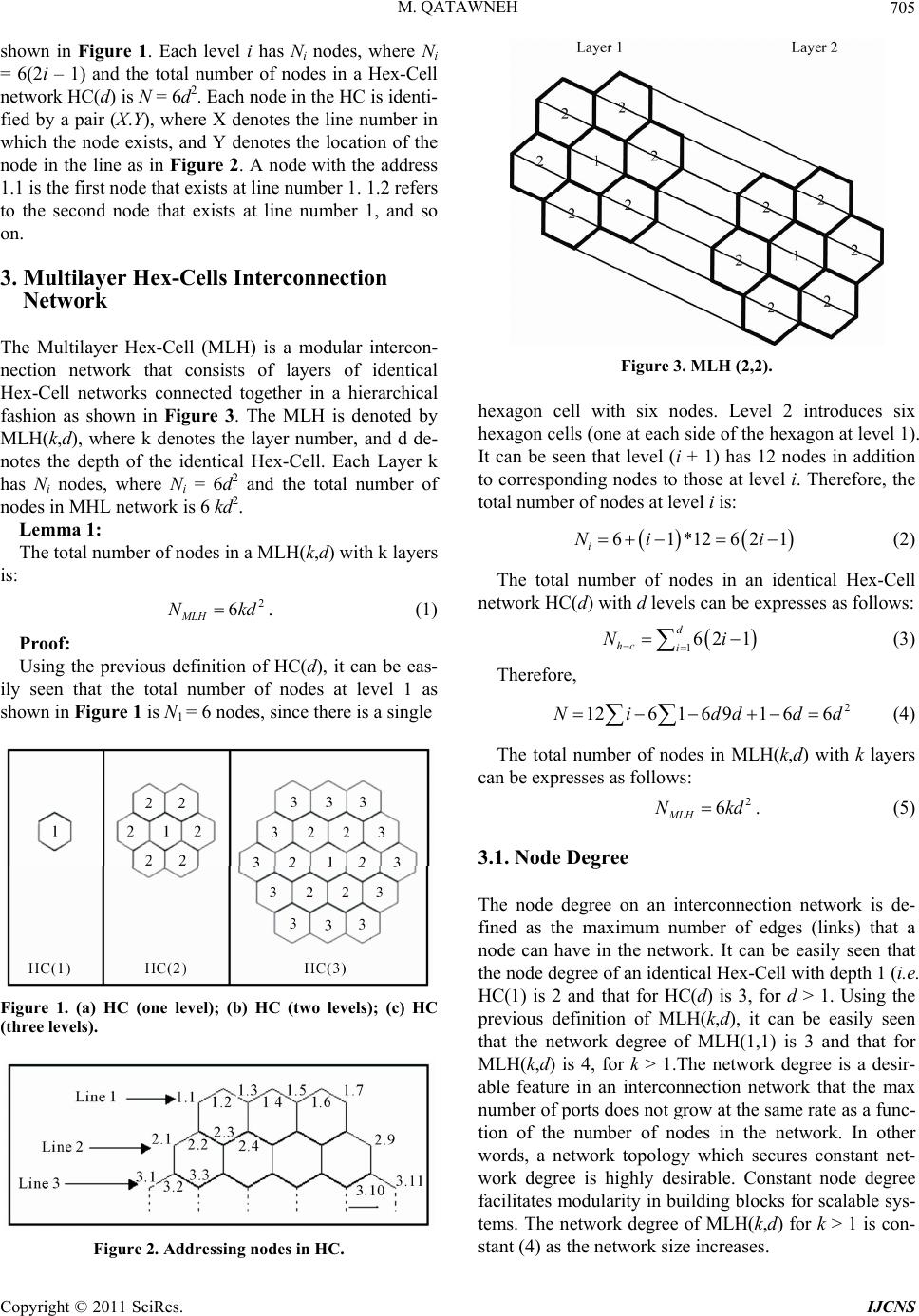
The following examples explain the above routing cases.
For this purposed, we consider a network of a MLH(2,2)
as shown in Figure 7.
Example 1: If (Ks < Kd).
Let (1.1.4) and (2.2.5) be the address of the source and
destination nodes respectively. CASE 3 of the routing
algorithm (i.e. source layer + 1) and moveDown will use
the following path: (2.1.4) → (2.1.5) → (2.2.5) as shown
in Figure 6. From Example 1, it can be easily seen that,
in order to forward a message to the next node, the rout-
ing algorithm performs only one operation (subtraction)
to the source layer (Ks – 1) and so on until the message
reaches its destination layer. When the source and desti-
nation layers are equal, the routing algorithm forwards
the message by applying the moveDown procedure as
shown in the Figure 7.
Example 2: If (Ks > Kd).
Let (2.3.7) and (1.1.4) be the address of the source and
destination nodes respectively. CASE 2 of the routing
algorithm (i.e. source layer –1) and moveUp will use the
following path: (1.3.7) → (1.2.7) → (1.2.6) → (1.1.5) →
(1.1.4) as shown in Figure 6. From Example 2, it can be
easily seen that, in order to forward a message to the next
node, the routing algorithm performs only one operation
(addition operation) to the source layer (Ks + 1) and so on
until the message reaches its destination layer. When the
source and destination layers are equal, the routing algo-
rithm forwards the message by applying the moveUp
procedure as shown in the Figure 7.
Example 3: If (Ks = Kd).
Let (1.4.5) and (1.4.1) be the address of the source and
destination nodes respectively.
CASE 1 of the routing algorithm (i.e. Ks = Kd). From
the address of the source and destination nodes, it is clear
that they are located at the same level (level 4). Applying
the routing algorithm the moveHorizontal will be used.
Figure 7. MLH(2,2).
The move Horizontal procedure will use the following
path: (1.4.4) → (1.4.3) → (1.4.2) → (1.4.1).
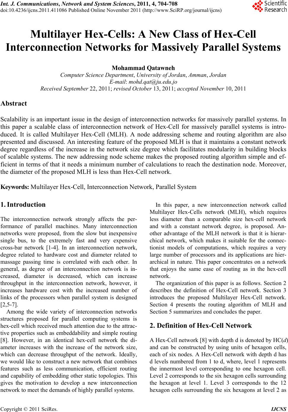
5. Conclusions
This paper introduced a new interconnection topology
called Multilayer Hex-Cells. Additionally, the paper
proposed an efficient routing algorithm for MLH which
requires no detailed knowledge of the network. The new
addressing node scheme makes the proposed routing
algorithm simple and efficient in terms of that it needs a
minimum number of calculations to reach the destination
node. The proposed MLH maintains a constant network
degree regardless of the increase in the network size de-
gree which facilitates modularity in building blocks of
scalable systems. Moreover, the diameter of the proposed
MLH is less than Hex-Cell.
While the proposed topology has been analyzed ma-
thematically and discussed through examples, it can be
tested as an underlining network for many applications in
distributed systems area.
6. References
[1] A. Mokhtar, “Multi-Level Hypercube Network,” Pro-
ceedings of the 5th International Conference in Parallel
Processing Symposium, Anaheim, 30 April - 2 May 1991,
pp. 475-480.
[2] S. Huyn, O. Jae-Chul and L. Hyeong-Ok, “Multiple Re-
duced Hypercube (MRH): A New Interconnection Net-
work Reducing Both Diameter and Edge of Hypercube,”
International Journal of Grid and Distributed Computing,
Vol. 3, No. 1, 2010, pp. 19-30.
[3] Y. Y. Liu and J. G. Han, “Double-Loop Hypercube: A
New Scalable Interconnection Network for Massively
Parallel Computing. Computing,” Proceedings of the
ISECS International Colloquium on Computing, Commu-
nication, Control, and Management, Guangzhou, 3-4 Au-
gust 2008, pp. 170-174. doi:10.1109/CCCM.2008.45
[4] T. Chan and Y. Saad, “Multigrid Algorithms on the Mul-
tiprocessor,” IEEE Transactions on Computers, Vol. C-35,
No. 11, 2002, pp. 969-977.
doi:10.1109/TC.1986.1676698
[5] S. Syed, K. Rizvi, M. Elleithy and A. Riasat, “An Effi-
cient Routing Algorithm for Mesh-Hypercube (M-H)
Networks,” Proceedings of the International Conference
on Parallel and Distributed Processing Techniques and
Applications, Las Vegas, 14-17 July 2008, pp. 69-75.
[6] C. Decayeux and D. Seme, “3D Hexagonal Network:
Modeling, Topological Properties, Addressing Scheme,
and Optimal Routing Algorithm,” IEEE Transaction on
Parallel and Distributed Systems, Vol. 16, No. 9, 2005,
pp. 875-884. doi:10.1109/TPDS.2005.100
[7] K. Day and A. Al-Ayyoub, “Topological Properties of
OTIS-Networks,” IEEE Transactions on Parallel and

M. QATAWNEH 708
Distributed Systems, Vol. 13, No. 4, 2002, pp. 359-366.
doi:10.1109/71.995816
[8] A. Sharieh, M. Qatawneh, W. Almobaideen and A. Sliet,
“Hex-Cell: Modeling, Topological Properties and Rout-
ing Algorithm,” European Journal of Scientific Research,
Vol. 22, No. 2, 2008, pp. 457-468.