A Real-Time Measurement Algorithm for Available Bandwidth

doi:10.4236/ijcns.2009.28086

Paper Menu >>

Journal Menu >>

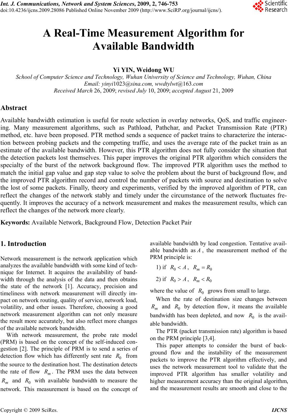Int. J. Communications, Network and System Sciences, 2009, 2, 746-753

doi:10.4236/ijcns.2009.28086 blished Online November 2009 (http://www.SciRP.org/journal/ijcns/).

A Real-Time Measurement Algorithm for

Available Bandwidth

Yi YIN, Weidong WU

School of Computer Science and Technology, Wuhan University of Science and Technology, Wuhan, China

Email: yinyi1023@sina.com, wwdtylwt@163.com

Received March 26, 2009; revised July 10, 2009; accepted August 21, 2009

Abstract

Available bandwidth estimation is useful for route selection in overlay networks, QoS, and traffic engineer-

ing. Many measurement algorithms, such as Pathload, Pathchar, and Packet Transmission Rate (PTR)

method, etc. have been proposed. PTR method sends a sequence of packet trains to characterize the interac-

tion between probing packets and the competing traffic, and uses the average rate of the packet train as an

estimate of the available bandwidth. However, this PTR algorithm does not fully consider the situation that

the detection packets lost themselves. This paper improves the original PTR algorithm which considers the

specialty of the burst of the network background flow. The improved PTR algorithm uses the method to

match the initial gap value and gap step value to solve the problem about the burst of background flow, and

the improved PTR algorithm record and control the number of packets with source and destination to solve

the lost of some packets. Finally, theory and experiments, verified by the improved algorithm of PTR, can

reflect the changes of the network stably and timely under the circumstance of the network fluctuates fre-

quently. It improves the accuracy of a network measurement and makes the measurement results, which can

reflect the changes of the network more clearly.

Keywords: Available Network, Background Flow, Detection Packet Pair

1. Introduction

Network measurement is the network application which

analyzes the available bandwidth with some kind of tech-

nique for Internet. It acquires the availability of band-

width through the analysis of the data and then obtains

the state of the network [1]. Accuracy, precision and

timeliness with network measurement will directly im-

pact on network routing, quality of service, network load,

volatility, and other issues. Therefore, choosing a good

network measurement algorithm can not only measure

the result more accurately, but also reflect more changes

of the available network bandwidth.

With network measurement, the probe rate model

(PRM) is based on the concept of the self-induced con-

gestion [2]. The principle of PRM is to send a series of

detection flow which has differently sent rate from

the source to the destination host. The destination detects

the rate of flow . The PRM uses the data between

and with available bandwidth to measure the

network. This measurement is based on the concept of

available bandwidth by lead congestion. Tentative avail-

able bandwidth as

, the measurement method of the

PRM principle is:

1) if AR



0, 0

RRm



2) if ,

AR 

0 0

RRm



where the value of grows from small to large.

When the rate of destination size changes between

and by detection flow, it means the available

bandwidth has been depleted, and now is the avail-

able bandwidth.

The PTR (packet transmission rate) algorithm is based

on the PRM principle [3,4].

This paper attempts to consider the burst of back-

ground flow and the instability of the measurement

packets to improve the PTR algorithm effectively, and

uses the network measurement tool to validate that the

improved PTR algorithm has smaller volatility and

higher measurement accuracy than the original algorithm,

and the measurement results are smooth and close to the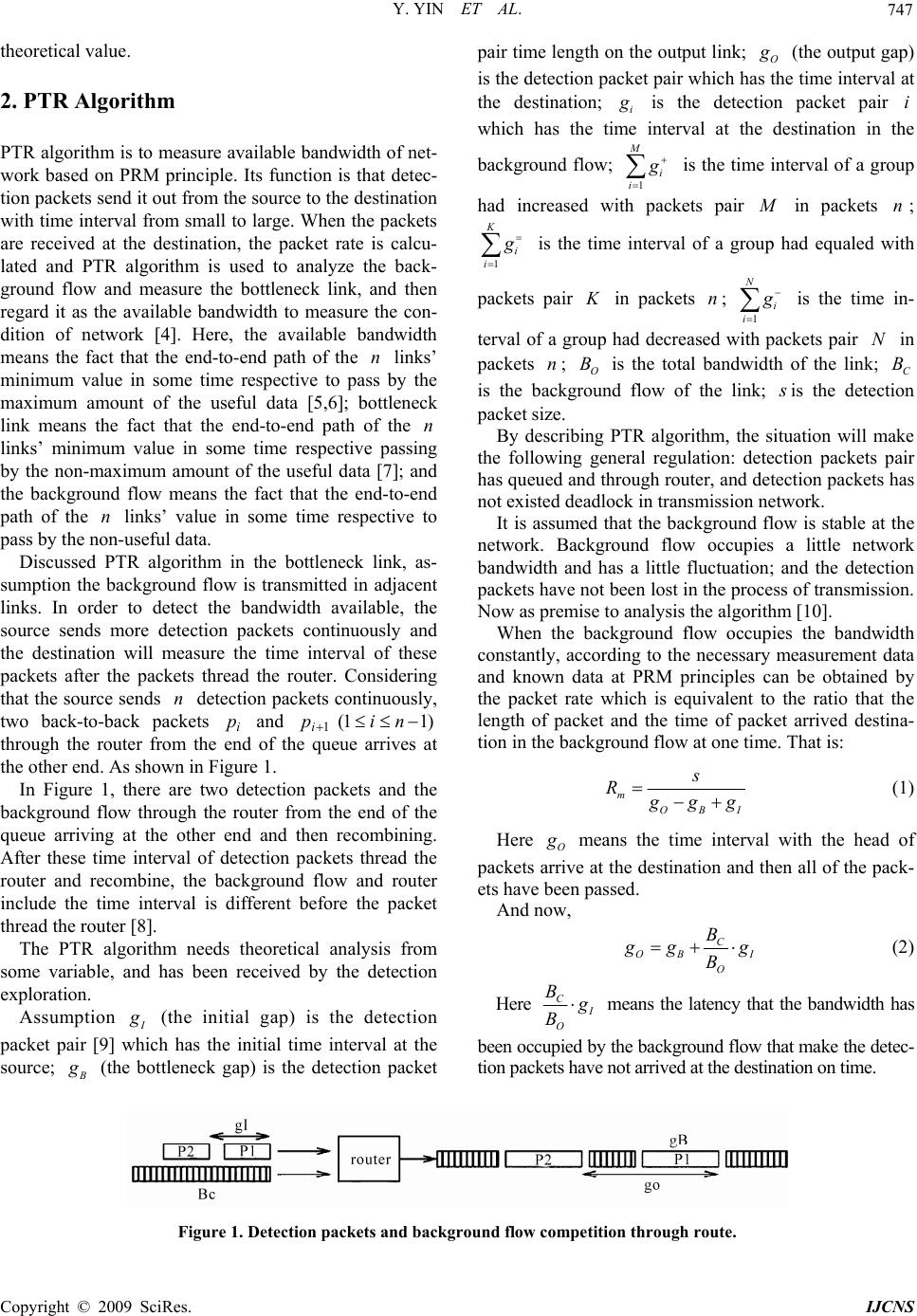

Y. YIN ET AL. 747

theoretical value.

2. PTR Algorithm

PTR algorithm is to measure available bandwidth of net-

work based on PRM principle. Its function is that detec-

tion packets send it out from the source to the destination

with time interval from small to large. When the packets

are received at the destination, the packet rate is calcu-

lated and PTR algorithm is used to analyze the back-

ground flow and measure the bottleneck link, and then

regard it as the available bandwidth to measure the con-

dition of network [4]. Here, the available bandwidth

means the fact that the end-to-end path of the links’

minimum value in some time respective to pass by the

maximum amount of the useful data [5,6]; bottleneck

link means the fact that the end-to-end path of the

links’ minimum value in some time respective passing

by the non-maximum amount of the useful data [7]; and

the background flow means the fact that the end-to-end

path of the links’ value in some time respective to

pass by the non-useful data.

Discussed PTR algorithm in the bottleneck link, as-

sumption the background flow is transmitted in adjacent

links. In order to detect the bandwidth available, the

source sends more detection packets continuously and

the destination will measure the time interval of these

packets after the packets thread the router. Considering

that the source sends detection packets continuously,

two back-to-back packets i and 1i

p p)11(





ni

through the router from the end of the queue arrives at

the other end. As shown in Figure 1.

In Figure 1, there are two detection packets and the

background flow through the router from the end of the

queue arriving at the other end and then recombining.

After these time interval of detection packets thread the

router and recombine, the background flow and router

include the time interval is different before the packet

thread the router [8].

The PTR algorithm needs theoretical analysis from

some variable, and has been received by the detection

exploration.

Assumption

(the initial gap) is the detection

packet pair [9] which has the initial time interval at the

source;

(the bottleneck gap) is the detection packet

pair time length on the output link; O

(the output gap)

is the detection packet pair which has the time interval at

the destination; i

is the detection packet pair

which has the time interval at the destination in the

background flow;







is the time interval of a group

had increased with packets pair

in packets ; n





is the time interval of a group had equaled with

packets pair

in packets n;





 is the time in-

terval of a group had decreased with packets pair in

packets ; is the total bandwidth of the link;

is the background flow of the link;

is the detection

packet size.

By describing PTR algorithm, the situation will make

the following general regulation: detection packets pair

has queued and through router, and detection packets has

not existed deadlock in transmission network.

It is assumed that the background flow is stable at the

network. Background flow occupies a little network

bandwidth and has a little fluctuation; and the detection

packets have not been lost in the process of transmission.

Now as premise to analysis the algorithm [10].

When the background flow occupies the bandwidth

constantly, according to the necessary measurement data

and known data at PRM principles can be obtained by

the packet rate which is equivalent to the ratio that the

length of packet and the time of packet arrived destina-

tion in the background flow at one time. That is:

OBI

 (1)

Here O

means the time interval with the head of

packets arrive at the destination and then all of the pack-

ets have been passed.

And now,



 (2)

Here C



means the latency that the bandwidth has

been occupied by the background flow that make the detec-

tion packets have not arrived at the destination on time.

Figure 1. Detection packets and background flow competition through route.

Y. YIN ET AL.

748

However, the background flow based on a constant of

bandwidth is only a basic situation that Equation (1)

cannot be used for the actual network. In general, back-

ground flow of bandwidth is always changing. The vari-

able bandwidth occupied by the background flow and the

rate of the detection packets arrival terminal is:

111

()

mMKN

iii

MKNs





 









(3)

Equation (3) as PTR equation, and PTR algorithm is

used by this equation.

The significance of this equation is the ratio that

sending a total length of several detection packets and

receiving all time of the detection packet at the destina-

tion of the link. According to the PRM principle, the

source rate will gain the network available bandwidth

information timely. The background flow, which has

occupied the bandwidth variably in the network, is the

application of measurement in the real situation.

Evidently, PTR algorithm is built on the PRM princi-

ple, which can be used by the changes of the background

flow and detected the packet rate.

3. Improved Algorithm

In the actual network measurement, either volatility or

loss detection packet has not been avoided. But the PTR

algorithm in measurement has not considered these two

issues. Therefore, it must remove these assumptions and

discuss verification in the actual network.

The original PTR algorithm, based on the PRM model,

has higher accuracy and faster speed of convergence

with the background flow relatively constant and the

utilization of the link is not high and the influence is

small for networks. As mentioned earlier that this is the

two assumptions of a description. When the flow is small

or stable with the network background flow traffic, de-

tection packet by the volatility of the time interval can be

more objective response network conditions. However,

when the network environment is poor, like the back-

ground flow changes on the network path, it is larger or

the utilization of the bottleneck link is higher, as back-

ground flow volatility is more obviously, the existing

PTR algorithm sends detection packets with the time

interval from small to large, which have some false

measurement value, and then the measurement results

significant ups and downs, which means the measure-

ment is not stable. As the detection packet is instable, it

cannot be obtained with accurate value when the network

condition has large fluctuation.

3.1. Theoretical Exploration with the Improved

Algorithm

Through Equation (3), the detection packet rate is the

ratio by two summations. Since the objective over PTR

algorithm reflects the changes in the bottleneck rather

than accurately to measure the timely rate with each detec-

tion packet, it can be arranged the PTR algorithm further.

Assumption detection packets will be divided into

groups once a time, each group has detection val-

ues. Firstly, calculate average send gap

() and average receive gap

() with the packet sequence i,

(

(gap

)__ isedavg

)__ gaprecavg

),0( k



). Secondly, calculate the summation of aver-

age send gap and average receive gap with the group of

packet sequence. The significance by Equation (3)

could be re-described

avgrecgapi







)

(4)

Apart from PTR algorithm over two data with i

and

, that needs to introduce two new values.

From the Equation (4), other than the interval time i

and the size

from the known detection packet with

the background flow at the source in Equation (3), it in-

troduces two new values, that are the average send

gap( ) and the average receive

gap().These two values mean the

weighted average with the time interval which is the

source and destination from the detection packets. As the

PTR algorithm does not measure the timely rate accu-

rately by detection packets, it only needs to measure the

changes of the network truly. It makes every time inter-

val values not accurate reflected, thus it just sum those

average value which could direct to reflect some

changes.

)(_ igapavg

)(_ igaprecavg

_sed

This methods estimate detection rates used to sample

mean can be reduced the consideration of the detection

packets that is not necessary to consider a small quantity

of the detection packets lost.

3.2. Improvement of the Algorithm in the

Circumstance of Frequent Fluctuations in

the Background Flow

Reference Equation (4) can improve the PTR algorithm

appropriately. Assumptions the detection packets have

been sent to the initial time interval init_gap and trans-

mitted to the time interval gap_step. init_gap and

gap_step will be set the fixed value but not as described

in the PTR algorithm from small to large to send the de-

tection packet with time interval [11].

Write algorithm for these conditions.

Algorithm PTR:

{

Y. YIN ET AL. 749

probe_num=PROBENUM;

packet_size=PACKETSIZE;

gB=GET_GB();

init_gap=gB/2;

gap_step=gB/8;

dst_gap_sum=0;

for(packet_size=PACKETSIZE;packet_size!=0;packet

_size--)

{

SEND_PROBING_PACKETS(probe_num;packet_size);

inc_gap_sum=GET_INCREASED_GAPS();

dst_gap_sum=GET_DST_GAPS();

}

c_bw=gB*inc_gap_sum/dst_gap_sum;

a_bw=b_bw-c_bw;

}

There are two fixed value in algorithm, that is,

init_gap=gB/2, gap_step=gB/8. These two values are

constant. When the gap values are constant, no matter

how changes in the network background flow, the band-

width is always constant over the detection packet.

Therefore, it is easy to be consistent with measurements

of the fluctuations and change of the background flow.

3.3. Improvement of the Algorithm in the

Circumstance of Desert with the Detection

Packets

If the original PTR algorithm encounters the high-inten-

sity in network background flow, as the total bandwidth

is always limited, even if the gap value is constant and

exploration data are nice match for the background flow,

detection packets may not arrival at the destination but

lost, thereby affect the analysis of the data. Analysis the

PTR equation, by the Equation (4) can be seen, if detec-

tion packet is lost, it will affect the convergence condi-

tions of the summation, thus affect the accuracy of the

detection data.

Now it describes the flow chart with improved PTR

algorithm, and increases the data with recording and con-

trolling in source and destination. At the same time, it

takes advantage of an improved approach to matching

the transmitter and receiver data, does accurate records,

and finally analyzes the network (Figure 2).

Source:

1) Take some group by detection packets from the host,

each group have packets, recorded as , where

],0[ kr



, deliver to send cache

2) Saving a constant time in send cache,

3) Deliver detection packet and from send cache,

then go 1)

Destination:

1) Waiting, record wait time at the same time

2) Receive detection packet from the source and

send it to receive cache, and intercalate a variable to

record the detection packets number from the source, the

initial value of is 0

3) Waiting time and detecting packet will be

handed over the host, and endue a new variable from

4) Go (1), then 0



R

5) Compare with , and define three value



M, 0



K, 0



N. If ,

sn tt

; if sn tt





; if sn tt





6) When the compare is complete,

0

It can be seen from the algorithm description to pro-

vide a very important parameter . With the value of

, it can be distinguished in the detection packets which

have been sent out to the destination, and the source is

arrived or lost due to the net reasons. If time is over, the

source without retransmission and the destination can

also automatically be received and recorded in the num-

ber of packets that insure match for the packets at each

side.

Figure 2. Flow chart with improved PTR algorithm.

Y. YIN ET AL.

750

Figure 3. Measurement topology.

Improving these two points by the original PTR algo-

rithm is that PTR algorithm is a method to change the

detection packets through its own to measure network.

This algorithm requires its own change to directly reflect

the network, but if the change of background flow is also

obviously, it is impossible to know the variation packets

are in congestion state. So the measurement result is de-

viation. At the same time, once the background flow is

too big, may lead the detection packets lost, which is

another reason to deviation of the measurement. These

deviations are PTR algorithm need to improve.

Improved algorithm, on the one hand, grasps the back-

ground flow of the changes is more accurately; on the

other hand, the transmission of detection packet hold

maximize control. Both of these improvements, the ac-

curacy of measurement have increased greatly, and the

changes of the load may too faster.

4. Experimental Results

First, using the improved PTR algorithm to measure

network, and calculate the theoretical data and circulate

algorithm to compare whether the results match. Second,

through network to analysis receive data to prove its pre-

cision and timeliness, and compare the original algorithm

to know the improved algorithm has higher accuracy.

Measurement topology as is shown in Figure 3.

is source and is destination above detection packet.

is monitor the variation in time interval with detec-

tion packet by source and is monitor by destination.

Monitor and compare data by two ends of the router

when detection packets have been sent. The topology of

experiments use the emulator [12], On this basis, com-

pare the original algorithm and the improved algorithm

with the theoretical value, and accord statistical proper-

ties of the Internet flow [13,14].

According to the Equation (4),

avgrecgapi



)

can be used in the algorithm to express the value of

, so

__dstgap sum

Rdstgap sumg











That acquire the output time interval O

. Compare

the measurement curves with the value of O

as is

shown in Figure 4, it also can reflect the basic values of

the network.

For msgB08.0



, , , msgI31.0 

BsMb /2.7

sMb /BO20



, the length of the detection packet is 700

Byte, and there are 60 packets in a group. Using the

emulator tools to make the background flow intensity

increased gradually from to . The

reason to take these values is whether it is time or rate

value, the size of these values are relatively modest

which have not been lost with changes in the quality of

network easily and have not been obliterated with the

sMb /0 s/Mb20

Figure 4. The theoretical value compared with the measured value.

Y. YIN ET AL. 751

Figure 5. The comparison of the value of receiving which are based on the same source rate between the original algorithm

and the improved algorithm.

excessive bandwidth facilely [4,15]. The theory is that

before the background flow intensity reached sMb /8.12

7 the detection packets

arrived at the destination will not obviously change

which have been sent. So, before the background flow

intensity reaches sMb /8.12, thn packets line

in the Figure 4 shows as a curve that the slope grows

slowly. When the background flow intensity from

M8.12 Mb0ction packet rate will slow

down gradually until the background flow can occupied

available bandwidth fully and causing bottlenecks that

lead to detection packets are inaccessible to destination.

At the destination, the detection rate of the available

bandwidth is . At this point in Figure 4, the rate

of the detection packets have been showed the curve that

the slope as . The measurements and theoretical

values inosculate basically. At the same time, the im-

proved algorithm compared to the original algorithm can

be clearly seen, the original algorithm with a strong vola-

tility, and the improved algorithm performance the value

have been smoothed. It is just consistent with the situa-

tion of the algorithm performance which after setting the

two fixed values in Caption 3.2 of the above described.

(sMb /20

sb /

sMb /2.

sMb /0



), the rate of

e detectio

to s, dete

According to the Equation (2), when the background

flow in the path and compete bandwidth with the detec-

tion packet flow, the output data stream for the time in-

terval is CI

gg B



 . This equation is going to be

validated with theoretical and experimental, and compare

the improved algorithm to the original algorithm, as is

shown in Figure 5.

Here, get . The remaining data with

the same on the past experimental data that the theoreti-

cal value is:

100 /

BMbs

7.2 0.31

0.08 0.10

100





In the experimental model, the source send detection

packets in the

C can be measured in the value of

in the 1

as shown in Figure 5 of the initial interval

value. When detection packets compete with background

flow which occupy the bandwidth to

though the router, the measurement value of the im-

proved PTR algorithm

7.2 /

BMbs

is as shown in Figure 5 with

the value “improved algorithm” in 2

, and the meas-

urement the same value of the original PTR algorithm as

is shown in Figure 5 with the value “original algorithm”.

The experimental results indicate that the improved algo-

rithm of the measurement results are nearly match with

the calculation results in Equation (2) , and the data from

the improved algorithm are more stable than original

algorithm.

The experiment result is proved the usefulness of the

detecting packets records as Caption 3.3.

The measurement result, which is gained by the ex-

perimental environment, and using the tool of MRTG

(Multi Router Traffic Grapher), compares with the im-

proved algorithm and the original algorithm. MRTG is a

software tool of monitoring network link flux load. It use

the snmp agrement to gain the flow information of the

equipment, and displays flux load to users by HTML

documents of graphics which included PNG format, dis-

playing the flux load in a very intuitive form. In the in-

terception 24-hour process of measurement, it has en-

tered 40Mb/s background flow for one hour initiatively,

but the intensity of other times background flow is only

20Mb/s. The measurement results are shown in Figure 6.

From the measurement results, we can see the measure-

ment results of improved algorithm and the stability of

MRTG are almost always the same and the improved

algorithm data are more stable than the original algo-

rithm data at the same time. Because the loss of detection

group is almost inevitable in the network, it has not

Y. YIN ET AL.

752

Figure 6. The original algorithm compete the same sending rate with the improved algorithm.

considered the factor of loss of detecting packets in

original algorithm. We can obtain the velocity of detect-

ing packets by data overall, the original algorithm would

produce some peak value as Figure 6 after detecting

group loss. The improved PTR algorithm, by dealing

with the lost detection packets, the results of detect is

more stable and accord with the measurement value

which was gained from MRTG.

When the background flow compete the whole band-

width with the data flow, the improved PTR algorithm

measure the data always accurate.

5. Conclusions

This paper discusses the theory and application of PTR

algorithm of network measurement. After the analysis of

the limitations and shortcomings of the algorithm, it

proposed the improved algorithm and processes, and by

comparing the algorithm’s theoretical value and the ac-

tual measured value to induce conclusions for perform-

ance improved algorithm can match with the theoretical

value better. At the same time, it also put up that im-

proved algorithm can measure the ins and outs of the

network accurately, increasing the veracity of the net-

work measuring and boosting up the precision of the

network measuring. Especially when the network speed

fluctuates frequently, it has a greater improvement in

reflecting of network conditions timely and accurately.

6. References

[1] S. Banerjee and A. Agrawala, “Estimating available ca-

pacity of a network connection [A],” IEEE International

Conference on Networks [C], Singapore, pp. 131–138,

September 2000. “NetDyn: Network Measutrements

Tool,” http://www.CS.umd.edu/suman/netdyn/.

[2] J. Strauss, D. Katabi, and F. Kaashoek, “A measurement

study of available bandwidth estimation tools [A],” Pro-

ceedings of ACM Intemet Measurement Conference

(IMC) [C], Miami Beach, Florida, October 2003.

[3] N. N. Hu and P. Steenkiste, “Evaluation and characteriza-

tion of available bandwidth probing techniques [J],”

IEEE Journal on Selected Areas in Communications, Vol.

21, No. 6, pp. 879–894, August 2003.

[4] C. Dovrolis, P. Ramanathan, and D. Moore, “What do

packet dispersion techniques measure?” in Proceedings of

Conference Computer Communication, pp. 905–914,

April 2001.

[5] M. Jain and C. Dovrofis, “End-to-end available band-

width: Measurement methodology, dynamics, and rela-

tion with TCP throughput [A],” Proceedings of ACM

SIGCOMM Symposium on Communication Architec-

tures Protocols [C], Pittsburgh, PA, USA, pp. 295–308,

August 2002.

[6] K. Lai and M. Baker, “Nettimer: A tool for measuring

bottleneck link bandwidth,” in Proceeding of USENIX

Symposium on Internet Technologies and Systems1, pp.

123–134, March 200.

[7] R. Prosad, C. Davrolis, M. Murray, et al., “Bandwidth

estimation: Metrics measurement techniques and tools

[J],” IEEE Network, Vol. 17, No. 6, pp. 27–35, 2003.

[8] V. Paxson, “Measurements and analysis of end-to-end

internet dynamics,” Ph. D. dissertation, Computer Sci-

ence Division, U. C. Berkeley, Berkeley, CA, May 1996.

[9] N. N. Hu and P. Steenkiste, “Estimating available band-

width using packet pair probing [J],” Carnegie Mellon

University (CMU), 9 September 2002.

[10] Pasztor A, Veitch D. The Packet Size Dependence of

Packet Pair Like Methods[C]. Proc. of IWQoS’ 02, Mi-

Y. YIN ET AL. 753

ami Beach, Florida, USA, 2002.

[11] Ns2 [Online]. Available: http://www.isi.edu/nsnam/ns.

[12] K. Claffy, G. Miller, and K. Thompson, “The nature of

the beast: Recent traffic measurements from an internet

backbone,” presented at the ISOC INET Conf., July

1998.

[13] Y. Zhang, N. Duffield, V. Paxson, and S. Shenker, “On

the constancy of Internet path properties,” in Proc. ACM

SIGCOMM Internet Measurement Workshop, San Fran-

cisco, CA, Nov. 2001, pp. 197–211.

[14] K. Claffy, G. Miller, and K. Thompson, “The nature of

the beast: Recent traffic measurements from an internet

backbone,” presented at the ISOC INET Conf., July

1998.