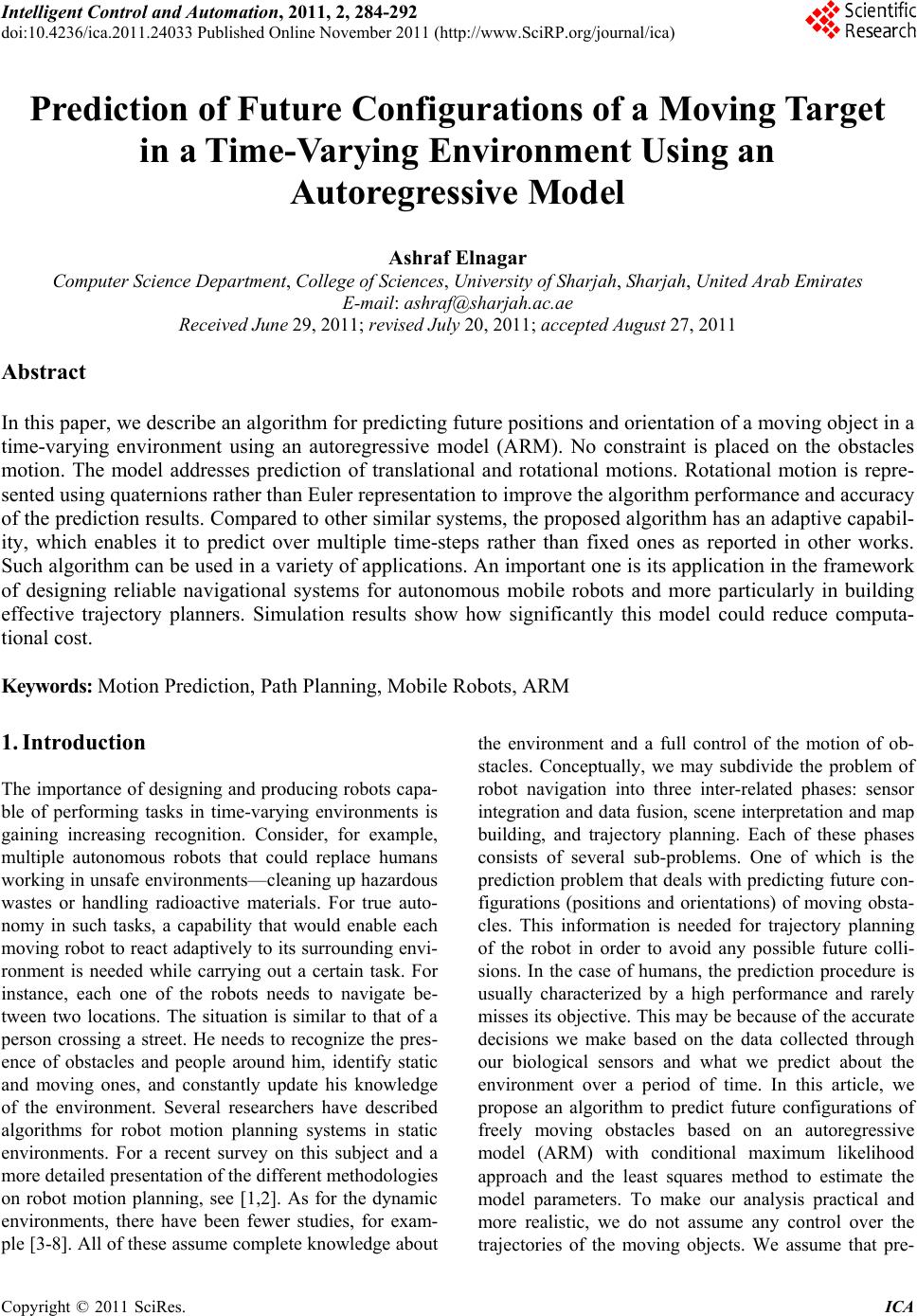
Intelligent Control and Automation, 2011, 2, 284-292
doi:10.4236/ica.2011.24033 Published Online November 2011 (http://www.SciRP.org/journal/ica)
Prediction of Future Configuration s of a Moving Target
in a Time-Varying Environment Using an
Autoregressive Model
Ashraf Elnagar
Computer Science Department, College of Sci ences , University of Sharjah, Sharjah, United Arab Emirates
Received June 29, 2011; revised July 20, 2011; accepted August 27, 2011
Abstract
In this paper, we describe an algorithm for predicting future positions and orientation of a moving object in a
time-varying environment using an autoregressive model (ARM). No constraint is placed on the obstacles
motion. The model addresses prediction of translational and rotational motions. Rotational motion is repre-
sented using quaternions rather than Euler representation to improve the algorithm performance and accuracy
of the prediction results. Compared to other similar systems, the proposed algorithm has an adaptive capabil-
ity, which enables it to predict over multiple time-steps rather than fixed ones as reported in other works.
Such algorithm can be used in a variety of applications. An important one is its application in the framework
of designing reliable navigational systems for autonomous mobile robots and more particularly in building
effective trajectory planners. Simulation results show how significantly this model could reduce computa-
tional cost.
Keywords: Motion Prediction, Path Planning, Mobile Robots, ARM
1. Introduction
The importance of designing and producing robots capa-
ble of performing tasks in time-varying environments is
gaining increasing recognition. Consider, for example,
multiple autonomous robots that could replace humans
working in unsafe environments—cleaning up hazardous
wastes or handling radioactive materials. For true auto-
nomy in such tasks, a capability that would enable each
moving robot to react adaptively to its surrounding envi-
ronment is needed while carrying out a certain task. For
instance, each one of the robots needs to navigate be-
tween two locations. The situation is similar to that of a
person crossing a street. He needs to recognize the pres-
ence of obstacles and people around him, identify static
and moving ones, and constantly update his knowledge
of the environment. Several researchers have described
algorithms for robot motion planning systems in static
environments. For a recent survey on this subject and a
more detailed presentation of the different methodologies
on robot motion planning, see [1,2]. As for the dynamic
environments, there have been fewer studies, for exam-
ple [3-8]. All of these assume complete knowledge about
the environment and a full control of the motion of ob-
stacles. Conceptually, we may subdivide the problem of
robot navigation into three inter-related phases: sensor
integration and data fusion, scene interpretation and map
building, and trajectory planning. Each of these phases
consists of several sub-problems. One of which is the
prediction problem that deals with predicting future con-
figurations (positions and orientations) of moving obsta-
cles. This information is needed for trajectory planning
of the robot in order to avoid any possible future colli-
sions. In the case of humans, the prediction procedure is
usually characterized by a high performance and rarely
misses its objective. This may be because of the accurate
decisions we make based on the data collected through
our biological sensors and what we predict about the
environment over a period of time. In this article, we
propose an algorithm to predict future configurations of
freely moving obstacles based on an autoregressive
model (ARM) with conditional maximum likelihood
approach and the least squares method to estimate the
model parameters. To make our analysis practical and
more realistic, we do not assume any control over the
trajectories of the moving objects. We assume that pre-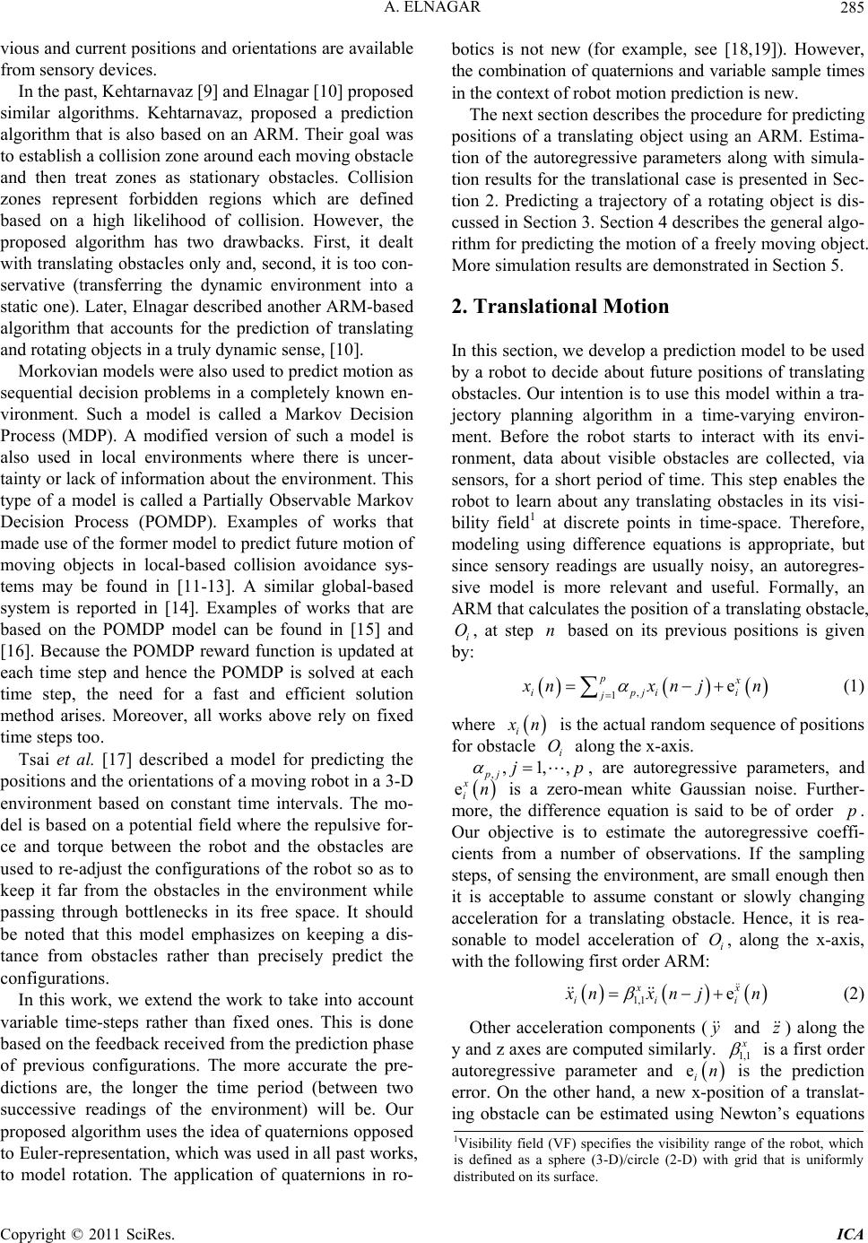

A. ELNAGAR285
i
vious and current positions and orientations are available
from sensory devices.
In the past, Kehtarnavaz [9] and Elnagar [10] proposed
similar algorithms. Kehtarnavaz, proposed a prediction
algorithm that is also based on an ARM. Their goal was
to establish a collision zone around each moving obstacle
and then treat zones as stationary obstacles. Collision
zones represent forbidden regions which are defined
based on a high likelihood of collision. However, the
proposed algorithm has two drawbacks. First, it dealt
with translating obstacles only and, second, it is too con-
servative (transferring the dynamic environment into a
static one). Later, Elnagar described another ARM-based
algorithm that accounts for the prediction of translating
and rotating objects in a truly dynamic sense, [10].
Morkovian models were also used to predict motion as
sequential decision problems in a completely known en-
vironment. Such a model is called a Markov Decision
Process (MDP). A modified version of such a model is
also used in local environments where there is uncer-
tainty or lack of information about the environment. This
type of a model is called a Partially Observable Markov
Decision Process (POMDP). Examples of works that
made use of the former model to predict future motion of
moving objects in local-based collision avoidance sys-
tems may be found in [11-13]. A similar global-based
system is reported in [14]. Examples of works that are
based on the POMDP model can be found in [15] and
[16]. Because the POMDP reward function is updated at
each time step and hence the POMDP is solved at each
time step, the need for a fast and efficient solution
method arises. Moreover, all works above rely on fixed
time steps too.
Tsai et al. [17] described a model for predicting the
positions and the orientations of a moving robot in a 3-D
environment based on constant time intervals. The mo-
del is based on a potential field where the repulsive for-
ce and torque between the robot and the obstacles are
used to re-adjust the configurations of the robot so as to
keep it far from the obstacles in the environment while
passing through bottlenecks in its free space. It should
be noted that this model emphasizes on keeping a dis-
tance from obstacles rather than precisely predict the
configurations.
In this work, we extend the work to take into account
variable time-steps rather than fixed ones. This is done
based on the feedback received from the prediction phase
of previous configurations. The more accurate the pre-
dictions are, the longer the time period (between two
successive readings of the environment) will be. Our
proposed algorithm uses the idea of quaternions opposed
to Euler-representation, which was used in all past works,
to model rotation. The application of quaternions in ro-
botics is not new (for example, see [18,19]). However,
the combination of quaternions and variable sample times
in the context of robot motion prediction is new.
The next section describes the procedure for predicting
positions of a translating object using an ARM. Estima-
tion of the autoregressive parameters along with simula-
tion results for the translational case is presented in Sec-
tion 2. Predicting a trajectory of a rotating object is dis-
cussed in Section 3. Section 4 describes the general algo-
rithm for predicting the motion of a freely moving object.
More simulation results are demonstrated in Section 5.
2. Translational Motion
In this section, we develop a prediction model to be used
by a robot to decide about future positions of translating
obstacles. Our intention is to use this model within a tra-
jectory planning algorithm in a time-varying environ-
ment. Before the robot starts to interact with its envi-
ronment, data about visible obstacles are collected, via
sensors, for a short period of time. This step enables the
robot to learn about any translating obstacles in its visi-
bility field1 at discrete points in time-space. Therefore,
modeling using difference equations is appropriate, but
since sensory readings are usually noisy, an autoregres-
sive model is more relevant and useful. Formally, an
ARM that calculates the position of a translating obstacle,
i, at step based on its previous positions is given
by:
On
 
,
1e
px
ipji
j
x
nxnj 


n (1)
where


i
x
nO
,1j
is the actual random sequence of positions
for obstacle along the x-axis.
i
,
,, pj p


, are autoregressive parameters, and


xnei is a zero-mean white Gaussian noise. Further-
more, the difference equation is said to be of order .
Our objective is to estimate the autoregressive coeffi-
cients from a number of observations. If the sampling
steps, of sensing the environment, are small enough then
it is acceptable to assume constant or slowly changing
acceleration for a translating obstacle. Hence, it is rea-
sonable to model acceleration of , along the x-axis,
with the following first order ARM:
p
i
O


1,1 e
x
iii

x
x
nxnj  

 n (2)
Other acceleration components (
y
 and ) along the
y and z axes are computed similarly. 1,1
z 
x

is a first order
autoregressive parameter and is the prediction
error. On the other hand, a new x-position of a translat-
ing obstacle can be estimated using Newton’s equations

nei
1Visibility field (VF) specifies the visibility range of the robot, which
is defined as a sphere (3-D)/circle (2-D) with grid that is uniformly
distributed on its surface.

A. ELNAGAR 286
of motion:
 
2
1
11 1
2
iini n
x
nxnxn txn t

 
 (3)
where and are the velocity and
acceleration of obstacle i along x-axis at step

1xn

 
1
i
xn

O


1n

,
respectively. n t

is the variable time interval between
and . The classical positional relationship
between acceleration and velocity along x-axis is:

1n

n
 


1
in
xn xn
xn t



 (4)
Substituting for

x
n
 and in (4) and then
equating Equation (2) with the result while substituting
for yields:

1xn



1
i
xn

 

 
1,1 1
1
21,11 1,1
12
1,1
2
(1 )1
(1 )
2
2e
x
nn
ii
n
xx
nnnn i
nn
xx nini
n
tt
xn xn
t
tttt xn
tt
txntn
t


 















 (5)
where 223nnn ttt


. Equation (1) is a 3rd order
ARM (compare with Equation (1)). Similarly, we can
predict the y and z coordinates of a translating object
along y and z-axes, respectively. In general the predic-
tion model for translational motion can be expressed in
the following matrix notation:





3,1 3,23,3
1
2e
3
i
ww ww
ii
i
wn
wnwnt n
wn
 
 









ni
 (6)
where


,,wxyz and the autoregressive coefficients
are:


1,1 1
1
1,1 1,1
3,1 3,23,3
12
1,1
2
1
1
T
w
nn
n
ww
ww w
nn
w n
n
tt
t
AB
tt
t
t



 


























where 2nn
A
tt



 and 2nn
A
tt



.
2.1. Estimating the Coefficients
To estimate the coefficients 3, (,1,2,3
jj)



using a
given sequence of data points that belong to obstacle
we need to minimize
 

1,2, ,
ii ii
Ox xxN




e,e
xy
ii
nn
 and


ez
in
 in Equation (6). There are
several approaches to do so. We present two of them.
The first one is the conditional maximum likelihood ap-
proach [20], [21] to estimate both the autoregressive co-
efficients and 2

, which is the variance of the noise.
The second model is based on the least squares method.
As for the first model, we will work the details of
minimizing


x
en

i only. The same procedure is used to
minimize the other error terms.





2
3;
33
22
x
cx
NN
 
3,1 3
2
2 3
3,
241
ln ln
1
2
xx
x
x
iji
kj
x
l,2 3, ,,
2π
N
x
kxkj











(7)
where N is the number of readings. To maximize the
logarithmic likelihood function (c), we differentiate
Equation (7) partially with respect to 3,1 3,23,3
l
,,
x
xx

 and
2
x

and equating the derivatives to zero. Note that for


3, we can only minimize the summation
part of Equation (7). However, looking again at Equation
(5) we notice that all
1,2, 3j
xj


’s are dependent on one coeffi-
cient 1,1
x

which can be determined from the following
conditional likelihood function [20]:



 

22
1,1
2
1,1
24
;l
N
j
x
33
n2πln
22
x
cx x
x
ii
NN
l
1
2
x
jxkj
 




 


2
,


0
(8)
where estimates should fall within the allowable range
1,1
11
x




 

 Note that (7) is the logarithm of
the conditional likelihood function for a third-order
autoregressive model whereas (8) represents the function
of a first-order model. Maximizing (8) with respect to
1,1
x

and 2
x

,we obtain:
 

 

4
2
4
4
4
ii
N
i
k
N
j
xk
xk
1,1
2
2
1,1
1
ˆ
1
ˆ
x
x
xi i
xk
1
N
k
x
jxkj





 
N






 
 (9)
Using 1,1
x

, we can easily determine the values of

’s in Equation (5) and consequently predict the future
position of a translating obstacle based on its history po-
sitions. The model needs at least four points before it
starts the prediction process. Compared with the first
approach (i.e., computing all
x

’s), the second one is
computationally inexpensive. It should be noted that the
estimates for the translational components along the y
and z axes can be obtained with the exact procedure de-
scribed earlier.
The second model which is widely used, [22], for es-

A. ELNAGAR287
timating the coefficient 1,1
x

as it changes with time, is
to fit an ARM to the sequence of acceleration in a least
squares sense as follows:


1,1 1,1
4
1,1
ˆarg min1
1
N
xt
ii
k
t
ii
xk xk
xk xk















 
 


1
where is a weight factor. For a uniformly
changing acceleration,

0  

is kept closer to 1. The solu-
tion to the above least squares problem is:
 
 
1,1 1,1
1
1
ˆˆ
1
1
tt t
t
ttt ii
tt tii
xtxt
xtxt








  
 
 
 
(10)
Similarly, we can obtain coefficients for translation
along the y and z axes. Notice the initial values for
and are set to 0. We used both models of estimating
coefficients in our simulation results. The second model
produces better results than the first model when pre-
dicting the motion of arbitrary moving objects. However,
the first model outperforms the second when predicting
for uniformly moving objects.
Δ
Ψ
2.2. Simulation Results: Translational Case
We introduce several simulation examples to show how
the proposed model works. In Figure 1 , we assume a 2D
work space in which a point-object is translating. Based
on its past positions, a predicted trajectory is generated
using the proposed ARM (dotted line). Each prediction
process is performed in a variable t

time. The closer
the dots are on the graph, the smaller the sampling time
is. If the prediction is accurate, the time interval of the
next reading is enlarged. The main difference between
the two graphs in Figures 1 and 2 is how the coefficient

is estimated? Figure 1 shows a predicted trajectory
of a translating point-object over a long period of time
(120 sampling steps) with varying acceleration. Although
the point does not follow a structured or well-defined2
trajectory, as in Figure 2, the predicted result (dotted line)
is quite close to the actual trajectory (solid line). The
mean square errors are 1.12 and 0.82 distance-units in
upper and lower graphs, respectively. A simulation in-
volving a well-defined trajectory (sin(x) curve) is dem-
onstrated in Figure 2. In this case, almost a perfect
match (mean square errors are 0.0016 and 0.0017 dis-
tance-units in upper and lower graphs, respectively) is
obtained between the actual and predicted future posi-
Figure 1. Predicting future positions based on (8) (upper
graph) and (9) (lower gr aph) for a moving point-object with
varying acceleration.
Figure 2. Predicting positions based on (8) (upper) and (9)
(lower) of a translating point-object with a uniform accel-
eration.
tions. While the upper graph of each figure shows the
result of using the conditional likelihood method [10],
the lower one depicts the result of using the least squares
technique [9]. The lower graph shows slightly better re-
sults in the case of varying acceleration. Comparing our
results to these two models ([19,10]) where prediction is
carried out based on a fixed time step, we did achieve as
good results based on the adaptive model but with less
time steps. For example, we obtained the results of Fig-
ures 1 and 2 in 88 and 99 steps, respectively, compared
to 120 and 360 steps when either of the systems of [10]
2A well-defined trajectory is one that can be modeled by a mathe-
matical function over a given time period.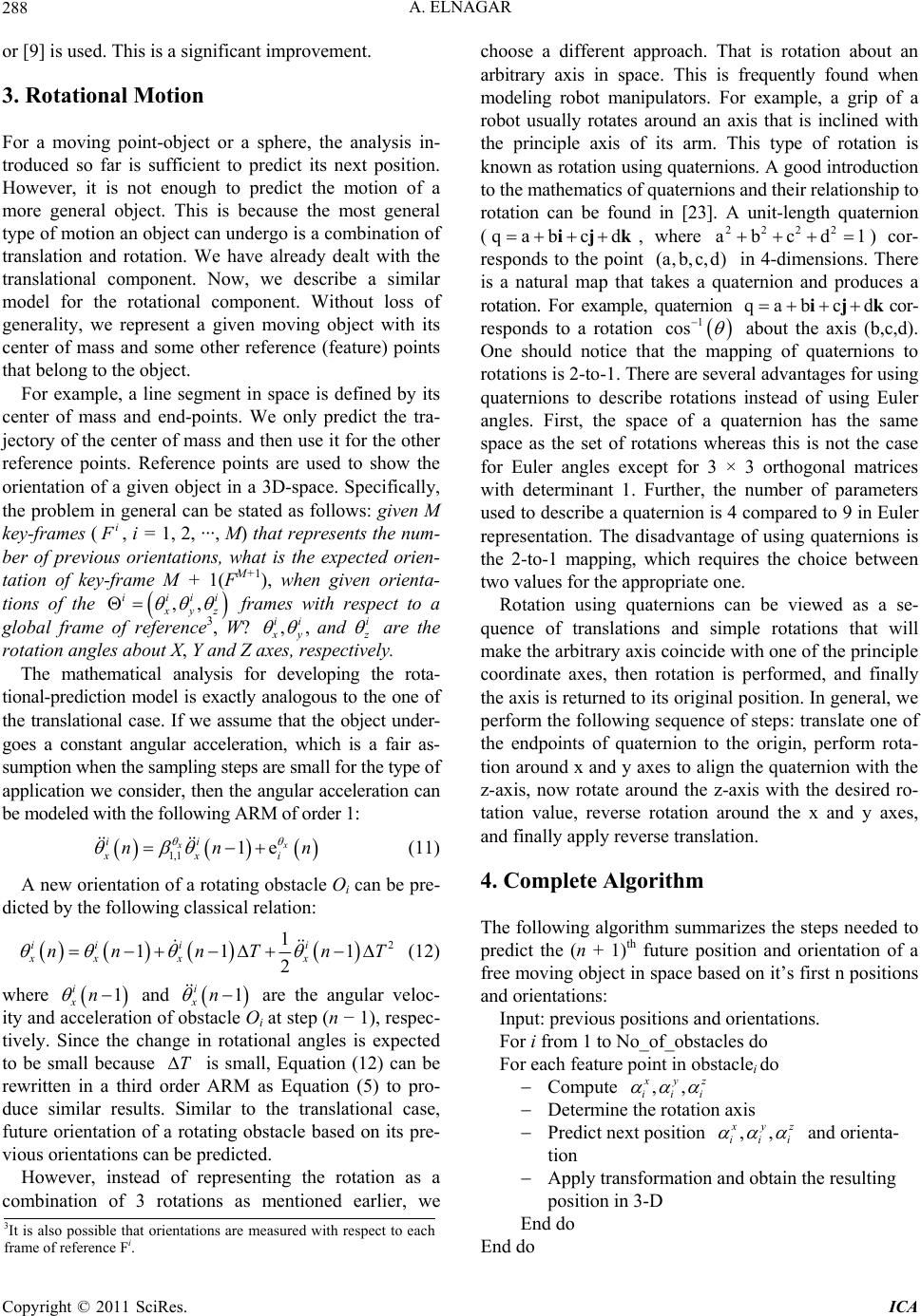

A. ELNAGAR 288
or [9] is used. This is a significant improvement.
3. Rotational Motion
For a moving point-object or a sphere, the analysis in-
troduced so far is sufficient to predict its next position.
However, it is not enough to predict the motion of a
more general object. This is because the most general
type of motion an object can undergo is a combination of
translation and rotation. We have already dealt with the
translational component. Now, we describe a similar
model for the rotational component. Without loss of
generality, we represent a given moving object with its
center of mass and some other reference (feature) points
that belong to the object.
For example, a line segment in space is defined by its
center of mass and end-points. We only predict the tra-
jectory of the center of mass and then use it for the other
reference points. Reference points are used to show the
orientation of a given object in a 3D-space. Specifically,
the problem in general can be stated as follows: given M
key-frames (i
F
, i = 1, 2, ···, M) that represents the num-
ber of previous orientations, what is the expected orien-
tation of key-frame M + 1(FM+1), when given orienta-
tions of the

,,
iiii

x
yz

  frames with respect to a
global frame of reference3, W? ,,
ii i
x
y
and z


x
n

are the
rotation angles about X, Y and Z axes, respectively.
The mathematical analysis for developing the rota-
tional-prediction model is exactly analogous to the one of
the translational case. If we assume that the object under-
goes a constant angular acceleration, which is a fair as-
sumption when the sampling steps are small for the type of
application we consider, then the angular acceleration can
be modeled with the following ARM of order 1:
 
1,11e
x
ii
xxi
nn

 
  (11)
A new orientation of a rotating obstacle Oi can be pre-
dicted by the following classical relation:
 
2
1
11 1
2
ii ii
xx xx
nnnTn   

T
 
(12)
where and are the angular veloc-
ity and acceleration of obstacle Oi at step (n − 1), respec-
tively. Since the change in rotational angles is expected
to be small because is small, Equation (12) can be
rewritten in a third order ARM as Equation (5) to pro-
duce similar results. Similar to the translational case,
future orientation of a rotating obstacle based on its pre-
vious orientations can be predicted.

1
i
xn
 

1
i
xn
 

T
However, instead of representing the rotation as a
combination of 3 rotations as mentioned earlier, we
choose a different approach. That is rotation about an
arbitrary axis in space. This is frequently found when
modeling robot manipulators. For example, a grip of a
robot usually rotates around an axis that is inclined with
the principle axis of its arm. This type of rotation is
known as rotation using quaternions. A good introduction
to the mathematics of quaternions and their relationship to
rotation can be found in [23]. A unit-length quaternion
(qabcd

ijk, where ) cor-
responds to the point in 4-dimensions. There
is a natural map that takes a quaternion and produces a
rotation. For example, quaternion cor-
responds to a rotation
2222
abcd 
d )
qab c
 ij

1
(a, b,c,
1
cos
d
k

 about the axis (b,c,d).
One should notice that the mapping of quaternions to
rotations is 2-to-1. There are several advantages for using
quaternions to describe rotations instead of using Euler
angles. First, the space of a quaternion has the same
space as the set of rotations whereas this is not the case
for Euler angles except for 3 × 3 orthogonal matrices
with determinant 1. Further, the number of parameters
used to describe a quaternion is 4 compared to 9 in Euler
representation. The disadvantage of using quaternions is
the 2-to-1 mapping, which requires the choice between
two values for the appropriate one.
Rotation using quaternions can be viewed as a se-
quence of translations and simple rotations that will
make the arbitrary axis coincide with one of the principle
coordinate axes, then rotation is performed, and finally
the axis is returned to its original position. In general, we
perform the following sequence of steps: translate one of
the endpoints of quaternion to the origin, perform rota-
tion around x and y axes to align the quaternion with the
z-axis, now rotate around the z-axis with the desired ro-
tation value, reverse rotation around the x and y axes,
and finally apply reverse translation.
4. Complete Algorithm
The following algorithm summarizes the steps needed to
predict the (n + 1)th future position and orientation of a
free moving object in space based on it’s first n positions
and orientations:
Input: previous positions and orientations.
For i from 1 to No_of_obstacles do
For each feature point in obstaclei do
 Compute ,,
x
yz
iii


 Determine the rotation axis
 Predict next position ,,
x
yz
iii

 and orienta-
tion
 Apply transformation and obtain the resulting
position in 3-D
End do
3It is also possible that orientations are measured with respect to each
frame of reference Fi. End do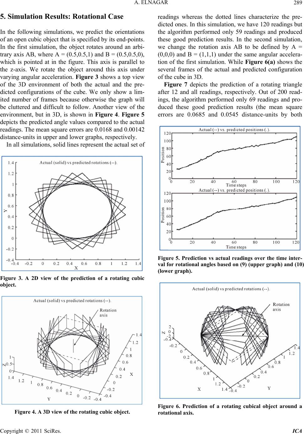

A. ELNAGAR289
5. Simulation Results: Rotational Case
In the following simulations, we predict the orientations
of an open cubic object that is specified by its end-points.
In the first simulation, the object rotates around an arbi-
trary axis AB, where A = (0.5,0.5,1) and B = (0.5,0.5,0),
which is pointed at in the figure. This axis is parallel to
the z-axis. We rotate the object around this axis under
varying angular acceleration. Figure 3 shows a top view
of the 3D environment of both the actual and the pre-
dicted configurations of the cube. We only show a lim-
ited number of frames because otherwise the graph will
be cluttered and difficult to follow. Another view of the
environment, but in 3D, is shown in Figure 4. Figure 5
depicts the predicted angle values compared to the actual
readings. The mean square errors are 0.0168 and 0.00142
distance-units in upper and lower graphs, respectively.
In all simulations, solid lines represent the actual set of
Figure 3. A 2D view of the prediction of a rotating cubic
object.
Figure 4. A 3D view of the rotating cubic object.
readings whereas the dotted lines characterize the pre-
dicted ones. In this simulation, we have 120 readings but
the algorithm performed only 59 readings and produced
these good prediction results. In the second simulation,
we change the rotation axis AB to be defined by A =
(0,0,0) and B = (1,1,1) under the same angular accelera-
tion of the first simulation. While Figure 6(a) shows the
several frames of the actual and predicted configuration
of the cube in 3D.
Figure 7 depicts the prediction of a rotating triangle
after 12 and all readings, respectively. Out of 200 read-
ings, the algorithm performed only 69 readings and pro-
duced these good prediction results (the mean square
errors are 0.0685 and 0.0545 distance-units by both
Figure 5. Prediction vs actual readings over the time inter-
val for rotational angles based on (9) (upper graph) and (10)
(low er graph).
Figure 6. Prediction of a rotating cubical object around a
rotational axis.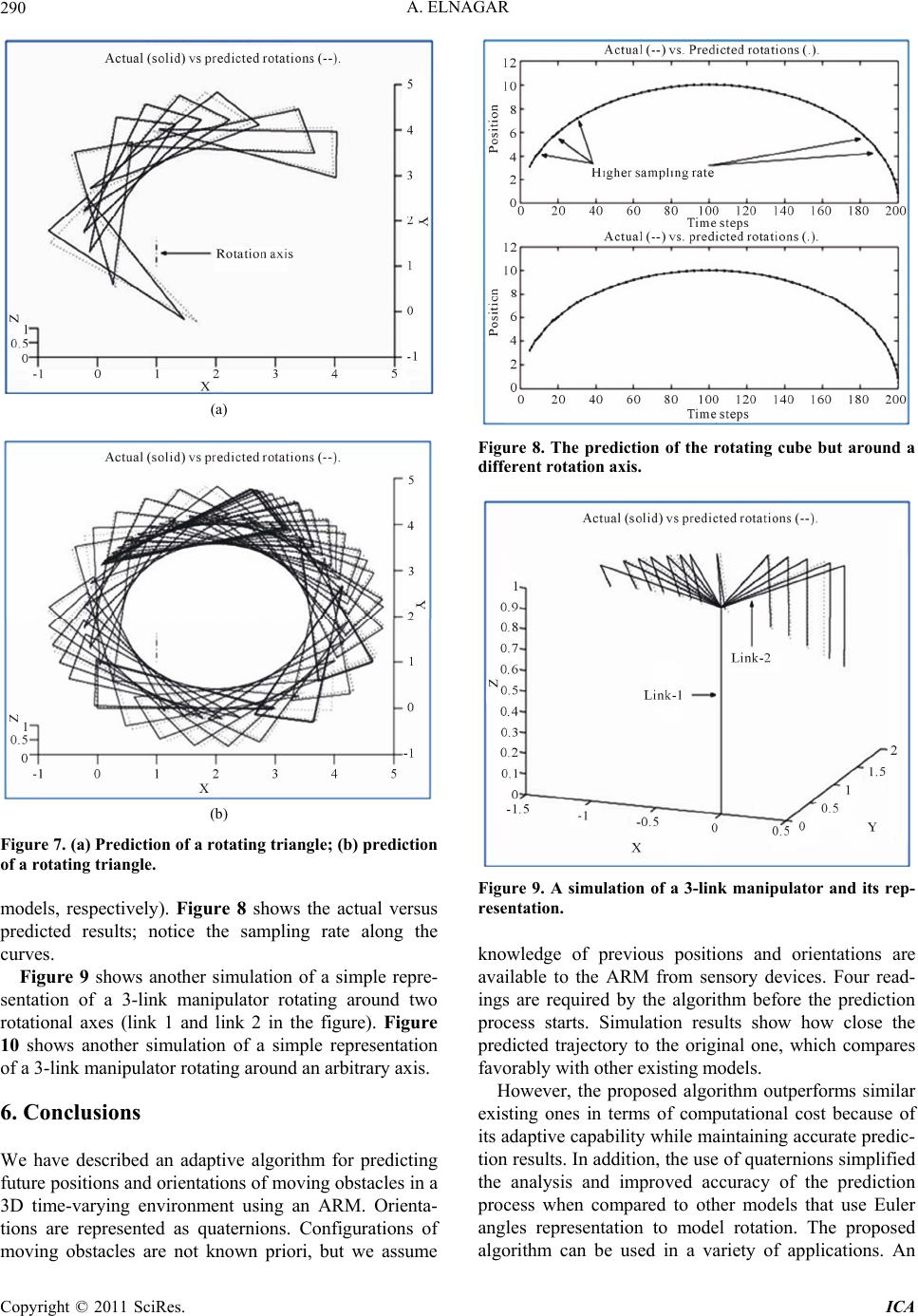

A. ELNAGAR 290
(a)
(b)
Figure 7. (a) Prediction of a rotating tria ngle ; (b) pre dic tio n
of a rotating triangle.
models, respectively). Figure 8 shows the actual versus
predicted results; notice the sampling rate along the
curves.
Figure 9 shows another simulation of a simple repre-
sentation of a 3-link manipulator rotating around two
rotational axes (link 1 and link 2 in the figure). Figure
10 shows another simulation of a simple representation
of a 3-link manipulator rotating around an arbitrary axis.
6. Conclusions
We have described an adaptive algorithm for predicting
future positions and orientations of moving obstacles in a
3D time-varying environment using an ARM. Orienta-
tions are represented as quaternions. Configurations of
moving obstacles are not known priori, but we assume
Figure 8. The prediction of the rotating cube but around a
different rotation axis.
Figure 9. A simulation of a 3-link manipulator and its rep-
resentation.
knowledge of previous positions and orientations are
available to the ARM from sensory devices. Four read-
ings are required by the algorithm before the prediction
process starts. Simulation results show how close the
predicted trajectory to the original one, which compares
favorably with other existing models.
However, the proposed algorithm outperforms similar
existing ones in terms of computational cost because of
its adaptive capability while maintaining accurate predic-
tion results. In addition, the use of quaternions simplified
the analysis and improved accuracy of the prediction
process when compared to other models that use Euler
angles representation to model rotation. The proposed
algorithm can be used in a variety of applications. An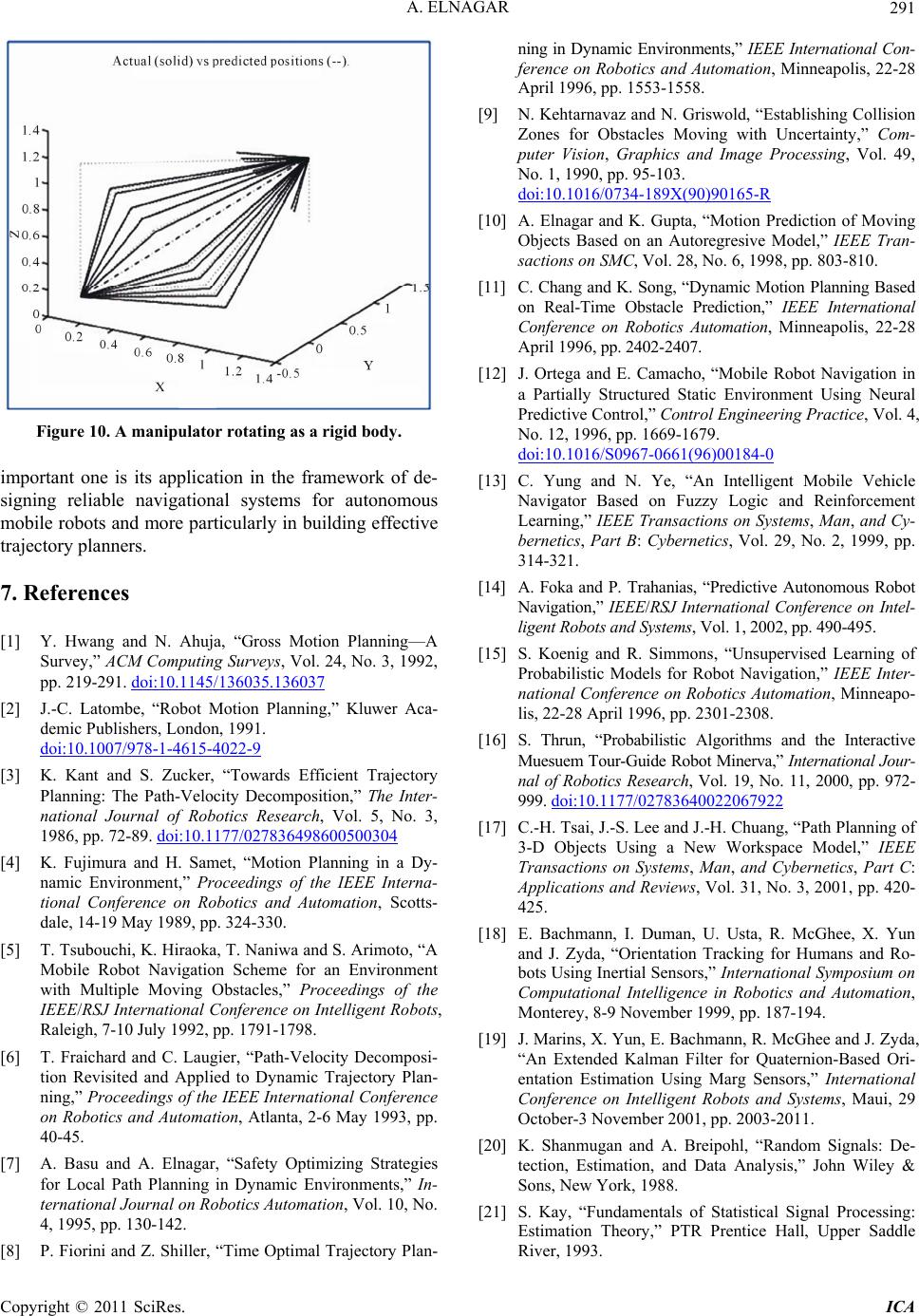

A. ELNAGAR291
Figure 10. A manipulator rotating as a rigid body.
important one is its application in the framework of de-
signing reliable navigational systems for autonomous
mobile robots and more particularly in building effective
trajectory planners.
7. References
[1] Y. Hwang and N. Ahuja, “Gross Motion Planning—A
Survey,” ACM Computing Surveys, Vol. 24, No. 3, 1992,
pp. 219-291. doi:10.1145/136035.136037
[2] J.-C. Latombe, “Robot Motion Planning,” Kluwer Aca-
demic Publishers, London, 1991.
doi:10.1007/978-1-4615-4022-9
[3] K. Kant and S. Zucker, “Towards Efficient Trajectory
Planning: The Path-Velocity Decomposition,” The Inter-
national Journal of Robotics Research, Vol. 5, No. 3,
1986, pp. 72-89. doi:10.1177/027836498600500304
[4] K. Fujimura and H. Samet, “Motion Planning in a Dy-
namic Environment,” Proceedings of the IEEE Interna-
tional Conference on Robotics and Automation, Scotts-
dale, 14-19 May 1989, pp. 324-330.
[5] T. Tsubouchi, K. Hiraoka, T. Naniwa and S. Arimoto, “A
Mobile Robot Navigation Scheme for an Environment
with Multiple Moving Obstacles,” Proceedings of the
IEEE/RSJ International Conference on Intelligent Robots,
Raleigh, 7-10 July 1992, pp. 1791-1798.
[6] T. Fraichard and C. Laugier, “Path-Velocity Decomposi-
tion Revisited and Applied to Dynamic Trajectory Plan-
ning,” Proceedings of the IEEE International Conference
on Robotics and Automation, Atlanta, 2-6 May 1993, pp.
40-45.
[7] A. Basu and A. Elnagar, “Safety Optimizing Strategies
for Local Path Planning in Dynamic Environments,” In-
ternational Journal on Robotics Automation, Vol. 10, No.
4, 1995, pp. 130-142.
[8] P. Fiorini and Z. Shiller, “Time Optimal Trajectory Plan-
ning in Dynamic Environments,” IEEE International Con-
ference on Robotics and Automation, Minneapolis, 22-28
April 1996, pp. 1553-1558.
[9] N. Kehtarnavaz and N. Griswold, “Establishing Collision
Zones for Obstacles Moving with Uncertainty,” Com-
puter Vision, Graphics and Image Processing, Vol. 49,
No. 1, 1990, pp. 95-103.
doi:10.1016/0734-189X(90)90165-R
[10] A. Elnagar and K. Gupta, “Motion Prediction of Moving
Objects Based on an Autoregresive Model,” IEEE Tran-
sactions on SMC, Vol. 28, No. 6, 1998, pp. 803-810.
[11] C. Chang and K. Song, “Dynamic Motion Planning Based
on Real-Time Obstacle Prediction,” IEEE International
Conference on Robotics Automation, Minneapolis, 22-28
April 1996, pp. 2402-2407.
[12] J. Ortega and E. Camacho, “Mobile Robot Navigation in
a Partially Structured Static Environment Using Neural
Predictive Control,” Control Engineering Practice, Vol. 4,
No. 12, 1996, pp. 1669-1679.
doi:10.1016/S0967-0661(96)00184-0
[13] C. Yung and N. Ye, “An Intelligent Mobile Vehicle
Navigator Based on Fuzzy Logic and Reinforcement
Learning,” IEEE Transactions on Systems, Man, and Cy-
bernetics, Part B: Cybernetics, Vol. 29, No. 2, 1999, pp.
314-321.
[14] A. Foka and P. Trahanias, “Predictive Autonomous Robot
Navigation,” IEEE/RSJ International Conference on Intel-
ligent Robots and Systems, Vol. 1, 2002, pp. 490-495.
[15] S. Koenig and R. Simmons, “Unsupervised Learning of
Probabilistic Models for Robot Navigation,” IEEE Inter-
national Conference on Robotics Automation, Minneapo-
lis, 22-28 April 1996, pp. 2301-2308.
[16] S. Thrun, “Probabilistic Algorithms and the Interactive
Muesuem Tour-Guide Robot Minerva,” Internati onal Jour-
nal of Robotics Research, Vol. 19, No. 11, 2000, pp. 972-
999. doi:10.1177/02783640022067922
[17] C.-H. Tsai, J.-S. Lee and J.-H. Chuang, “Path Planning of
3-D Objects Using a New Workspace Model,” IEEE
Transactions on Systems, Man, and Cybernetics, Part C:
Applications and Reviews, Vol. 31, No. 3, 2001, pp. 420-
425.
[18] E. Bachmann, I. Duman, U. Usta, R. McGhee, X. Yun
and J. Zyda, “Orientation Tracking for Humans and Ro-
bots Using Inertial Sensors,” International Symposium on
Computational Intelligence in Robotics and Automation,
Monterey, 8-9 November 1999, pp. 187-194.
[19] J. Marins, X. Yun, E. Bachmann, R. McGhee and J. Zyda,
“An Extended Kalman Filter for Quaternion-Based Ori-
entation Estimation Using Marg Sensors,” International
Conference on Intelligent Robots and Systems, Maui, 29
October-3 November 2001, pp. 2003-2011.
[20] K. Shanmugan and A. Breipohl, “Random Signals: De-
tection, Estimation, and Data Analysis,” John Wiley &
Sons, New York, 1988.
[21] S. Kay, “Fundamentals of Statistical Signal Processing:
Estimation Theory,” PTR Prentice Hall, Upper Saddle
River, 1993.

A. ELNAGAR 292
[22] M. Shensa, “Recursive Least Squares Lattice Algorithms—
A Geometric Approach,” IEEE Transactions on Auto-
matic Control, Vol. 26, No. 3, 1981, pp. 695-702.
doi:10.1109/TAC.1981.1102682
[23] K. Shoemake, “Animating Rotations with Quaternion Cur-
ves,” Computer Graphics, Vol. 19, No. 3, 1985, pp. 245-
254. doi:10.1145/325165.325242