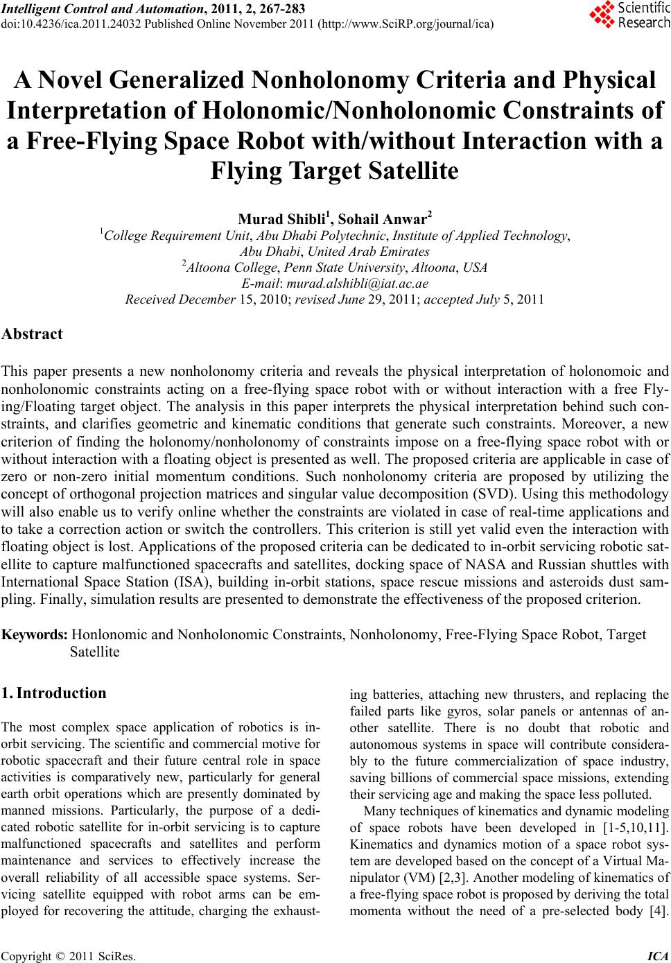Intelligent Control and Automation, 2011, 2, 267-283
doi:10.4236/ica.2011.24032 Published Online November 2011 (http://www.SciRP.org/journal/ica)
A Novel Generalized Nonholonomy Criteria and Physical
Interpretation of Holonomic/Nonholonomic Constraints of
a Free-F lyin g S pac e R obo t w ith /without Interaction with a
Flying Target Satellite
Murad Shibli1, Sohail Anwar2
1College Requirement Unit, Abu Dhabi Polytechnic, Institute of Applied Technology,
Abu Dhabi, United Arab Emirates
2Altoona College, Pen n St a t e U ni ve rsi ty, Altoona, USA
Received December 15, 2010; revised June 29, 2011; accepted July 5, 2011
Abstract
This paper presents a new nonholonomy criteria and reveals the physical interpretation of holonomoic and
nonholonomic constraints acting on a free-flying space robot with or without interaction with a free Fly-
ing/Floating target object. The analysis in this paper interprets the physical interpretation behind such con-
straints, and clarifies geometric and kinematic conditions that generate such constraints. Moreover, a new
criterion of finding the holonomy/nonholonomy of constraints impose on a free-flying space robot with or
without interaction with a floating object is presented as well. The proposed criteria are applicable in case of
zero or non-zero initial momentum conditions. Such nonholonomy criteria are proposed by utilizing the
concept of orthogonal projection matrices and singular value decomposition (SVD). Using this methodology
will also enable us to verify online whether the constraints are violated in case of real-time applications and
to take a correction action or switch the controllers. This criterion is still yet valid even the interaction with
floating object is lost. Applications of the proposed criteria can be dedicated to in-orbit servicing robotic sat-
ellite to capture malfunctioned spacecrafts and satellites, docking space of NASA and Russian shuttles with
International Space Station (ISA), building in-orbit stations, space rescue missions and asteroids dust sam-
pling. Finally, simulation results are presented to demonstrate the effectiveness of the proposed criterion.
Keywords: Honlonomic and Nonholonomic Constraints, Nonholonomy, Free-Flying Space Robot, Target
Satellite
1. Introduction
The most complex space application of robotics is in-
orbit servicing. The scientific and commercial motive for
robotic spacecraft and their future central role in space
activities is comparatively new, particularly for general
earth orbit operations which are presently dominated by
manned missions. Particularly, the purpose of a dedi-
cated robotic satellite for in-orbit servicing is to capture
malfunctioned spacecrafts and satellites and perform
maintenance and services to effectively increase the
overall reliability of all accessible space systems. Ser-
vicing satellite equipped with robot arms can be em-
ployed for recovering the attitude, charging the exhaust-
ing batteries, attaching new thrusters, and replacing the
failed parts like gyros, solar panels or antennas of an-
other satellite. There is no doubt that robotic and
autonomous systems in space will contribute considera-
bly to the future commercialization of space industry,
saving billions of commercial space missions, extending
their servicing age and making the space less polluted.
Many techniques of kinematics and dynamic modeling
of space robots have been developed in [1-5,10,11].
Kinematics and dynamics motion of a space robot sys-
tem are developed based on the concept of a Virtual Ma-
nipulator (VM) [2,3]. Another modeling of kinematics of
a free-flying space robot is proposed by deriving the total
momenta without the need of a pre-selected body [4].

M. SHIBLI ET AL. 268
While in [5] the kinematics of a free-flying multi-body
system is investigated by introducing the conservation of
momentum and deriving a new Jacobian matrix called
the Generalized Jacobian. In research [6], the kinematics
and dynamics of free-floating coordinated space robotic
system with closed kinematic constraints are developed.
An approach to position and force control of free-float-
ing coordinated space robots with closed kinematic con-
straints is proposed for the first time. Unlike previous
coordinated space robot control methods which are for
open kinematic chains, the method presented here ad-
dresses the main difficult problem of control of closed
kinematic chains. The controller consists of two parts,
position controller and internal force controller, which
regulate, respectively, the object position and internal
forces between the object and end-effectors. A planar
FFSR with a 2 DOFs manipulator is selected to test the
algorithm and simulation results illustrate that the path
following is realized precisely. The genetic algorithm
with wavelet approximation is applied to nonholonomic
motion planning in [7]. The problem of nonholonomic
motion planning is formulated as an optimal control
problem for a drift.
When a robot end-effecter interacts with a stationary
environment or moving object, it imposes a geometric
holonomic (integrable) constraint [2,9,11]. The conser-
vation of momentum exerts kinematic-like constraints on
a space robot in the absence of external forces. The linear
momentum is considered as holonomic but the angular
momentum as nonholonomic (non-integrable) [11]. Con-
trol of nonholonomic system received a great attention of
the research developed in [8,11-13,14]. Research [15]
addresses modeling, simulation and controls of a robotic
servicing system for the hubble space telescope servicing
missions. The simulation models of the robotic system
include flexible body dynamics, control systems and
geometric models of the contacting bodies. These models
are incorporated into MDA’s simulation facilities, the
multibody dynamics simulator “space station portable
operations training simulator (SPOTS)”. In [16], the
kinematics of the FFSR is introduced firstly. Then the
null space approach is used to reparameterize the path:
the direction and magnitude are decoupled and no direc-
tion error is introduced. And the Newton iterative me-
thod is adopted to find the optimal magnitude of the joint
velocity. The inverse kinematic control based on mutual
mapping neural network of free-floating dual-arm space
robot system without the basepsilas control is discussed
in [17]. With the geometrical relation and the linear, an-
gular momentum conservation of the system, the gener-
alized Jacobian matrix is obtained.
To solve the challenge of nonintegrability of principle
of conservation of angular momentum many researchers
have proposed different schemes. A nonholonomic path
planning of space robots is proposed in [8] via bi-direc-
tional approach. The spacecraft orientation can be con-
trolled in addition to the joint variables of the manipula-
tor, by actuating only the joint variables, if the trajectory
is carefully planned. A major characteristic of a space
robot is clearly the distinction from ground-based robot
is the lack of a fixed base in space environment [5].
Since the conservation of momentum exerts kinematic-
like constraints on a space robotic system in the absence
of external forces, one may raise the question: what is the
physical interpretation of such a behavior? Some re-
searchers have looked at this problem from trajectory
planning point of view, From trajectory planning point of
view, not all trajectories and displacements (velocities)
are allowed due to the conservation of momentum and
geometric constraints [8,11]. The physical meaning be-
hind these constraints is that they restrict the kinemati-
cally possible displacements (possible values of the ve-
locities) of the individual parts of the system.
The physical characteristics of the nonholonomic con-
straints are exhibited by the fact that even if the manipu-
lator joints return to their initial configuration after a
sequence of motion, the vehicle orientation may not be
the same as the initial value [8]. If a space robot is oper-
ated in a certain task, position and attitude of the base
satellite are disturbed by reaction forces and moments
due to the robot motion, so it cannot accomplish a task
without provision for this disturbance. No space ma-
nipulator can avoid the reaction disturbance. Physical
interpretation of such behavior will give us more idea
about the nature of holonomic and nonholonomic con-
straints and geometric conditions that generate those
constraints. Verifying the intergrability of holonomic and
nonholnomic constrained systems has attracted the atten-
tion of several studies [8-18]. Frobenius theorem is a well-
known approach to answer the question of integrability
of such systems under concern. Conditions of the inte-
grability of nonholonomic systems are reported using Lie
algebra techniques in [8]. A necessary and sufficient
condition is reported by using what is called bilinear co-
variants in [12,13-18]. Nonholomic behavior of a free-
flying space robot is investigated in the absence of ex-
ternal forces by Lie algebra techniques [8]. Differen-
tial-form-based integrability conditions for dynamic con-
straints using the Frobenius theorem are proposed in [19].
In the latter, the conditions can be used for the classifica-
tion of holonomic and nonholonomic constraints. Unfor-
tunately, using Lie algebra and bilinear covariant is cum-
bersome and time consuming in the case of complicated
space robotic systems.
This paper presents a new methodology to determine
holonomy/nonholonomy of constraints impose on a free-

M. SHIBLI ET AL.269
flying space robot with or without interaction with a
floating object. In this work a physical interpretation of
nonholnomic constraints is presented. It gives an insight
of nonholonomic constraints and provides more informa-
tion of a space robot behavior, especially in control
which is more difficult than conventional holonomic
systems. The holonomy criterion is proposed by utilizing
the concept of orthogonal projection matrices and singu-
lar value decomposition (SVD). This criteria is economic
(from computational view point) can easily be used to
verify the holonomy of a space robot exposed to different
types of constraints. Using this methodology will also
enable us to verify online whether the constraints or their
initial conditions are violated in case of real-time appli-
cations and to take a corrective action or switch the con-
trollers if needed. Such a physical interpretation will
provide us with a better understanding of a space robot
especially in contact task planning and control, which are
more difficult than conventional holonomic systems.
The paper is organized as follows: In Section 2, mod-
eling of kinematics, linear and angular momentum are
derived. In Section 3, a physical interpretation of non-
holnomic constraints is presented. In Section 4, non-
holonomy criteria in case of zero initial momentum con-
ditions, meanwhile in Section 5 a nonholonomy criteria
of non-zero initial momentum conditions space robotic
system is presented. Finally, simulation results and con-
clusions are presented respectively in Sections 6 and 7 to
demonstrate the analytical results.
2. Kinematics and Momentum Modeling
2.1. Nomenclature
All generalized coordinates are measured in the inertial
frame unless another frame is mentioned as follows:
i
m: the mass of the ith body;
3
i
I
Rn
qR
: the inertia of the ith body;
: the robot joint variable vector q(q1, q2, ···, qn)T;
3
RR
b3
RR
: the position vector of the centroid of the base;
T3
rR
: the position vector of the target satellite;
i: the position vector of the ith joint;
3
TEE R
f
and the
R: the position vector of the target satellite
centroid with respect to the end-effecter (EE);
3
b
VR
3
R
: the linear velocity of the base;
b
U: the base angular velocity vector;
3: the identity matrix. 33
2.2. Kinematics
The purpose of this part is to model the kinematics of a
free-flying space robotic manipulator in contact with a
captured satellite as a whole. In this model the contact
between the space robot and the target satellite is as-
sumed established and not escaped.
Our combined system can be modeled as a multi-body
chain system composed o2 rigid bodies. While
the manipulator links are numbered from 1to n, the
base satellite (body 0) is denot by b, in particular,
n
ed


1thn body (the target satellite) by T.
Moreover, This multi-body system is connecty 1n ed b

joints, which are given numbers from 11n to

. Where
the end-effecter is represented as the joint as
shown in Figure 1.

n

1th
We assume that all system bodies are rigid, the contact
surfaces are frictionless and known. Also the effect of
gravity gradient, solar radiation and aerodynamic forces
are weak and neglected. It is assumed also that the base
satellite is reaction-wheel actuated.
Referring to Figure 1, the position vector of the ith
body centroid with respect to the inertial frame can be
expressed as [20-22]
ibi
RRR
b

 (1)
where the relative vector ib
R is the position of the ith
body centroid with respect to the base frame.
Upon differentiating both sides of (1) with respect to
time, the relationship between the ith body velocity
Figure 1. Multi-body diagram of a free-floating space robot
in contact with a target satellite.

M. SHIBLI ET AL. 270
ib bib
VVR v 
i
(2)
where i is the linear velocities of the ith body in base
coordinates. Now in the case of any ith body of the ma-
nipulator, the velocity i can be expressed in terms of
the linear Jacobian matrix as
v
v
i
iL
vJq (3)
where






112 2
,,,,0,
i
Li iiii
JzRrzRr zRr   

,0
(4)
The end-effecter tip velocity is given by
EE
EEbbEE bL
VVR J  q
(5)
Additionally, the velocity T of the target satellite in
the reference frame can be obtained by deriving Equation
applying (1) as
V
T
TbbTbL TTEE
VVR JqRv   
T (6)
Since the target satellite is not stationary, (6) shows
the relative linear and angular velocities T, T v

be-
tween the end effecter and the target satellite and meas-
ured in the base frame.
Another relationship is needed between the ith body
angular velocity and joint angular velocity
i

ibi

 (7)
where i

is the angular velocities of the ith body in
base coordinates and i

in case of the manipulator is
given by
i
iA
J
q   (8)
where the angular Jacobian


12
,,,,0,,0
i
Ai
Jzzz (9)
While in the case of the target satellite, the absolute
angular velocity of can be expressed as
EE
TbA
Jq T

 
 (10)
2.3. Linear and Angular Momentum
The linear and angular momentum of a multi-body sys-
tem is a key part in understanding the motion of the sys-
tem when it is not subjected to external forces. They may
impose kinematic-like constraints when the system is
free of any external force.
The linear momentum and angular momentum
of the whole system is given by
P L
1
0
n
ii
i
Pm


V

V
(11)

1
0
nBiiii i
i
LImR



 (12)
By means of (1)-(10), linear and angular momentum in
(11)-(12) can then be represented in a compact form as
bbb b
Vb b
bb
bT bT
bT bT
VV Vq
b
Tbq
VVv
T
T v
MM M
V Pq
MM
LM
MM
v MM











 

  
   










(13)
where each block of the matrix is defined as follows
133
3
0
b
n
Vi
i
M
UmR



 (14)
133
0,
bb
n
Viib
iib
M
mR R


  

 (15)
13
0,
bi
nn
Vqi L
iib
M
mJ R



 (16)
 
133
0,
b
n
ii ibb
iib
M
ImDRI R


 
 (17)


13
0,
biL
i
n
B
n
qiAiib
iib
M
IJm RJR







(18)
33
1
bT
VnTEE
M
mR R



 
 (19)


33
1
bT
b
iTEE n
M
mD RIR





 (20)
33
31
bT
Vv n
M
Um R


(21)


33
11
bT
vnn
M
mR R


  (22)
Note that the matrix function


R for a vector
,, T
xyz
RRRR




 is defined as

33
0
0
0
zy
zx
yx
RR
RR RR
RR



  






3
(23)
and
 
22
22 3
22
T
yz xyxz
xyx zyz
xzyzxy
DR RR
RR RRRR
RRR RRRR
RRRRR R

 

 

 


 

(24)
and the sub-matrices of the Jacobian of the ith body rep-
resenting the linear and angular parts are defined before.
Note that as in (13) the system is subjected to a non-
holonomic (non-integrable) constraint because of con-
servation of angular momentum in the absence of exter-
nal forces. On the contrast, the linear momentum results

M. SHIBLI ET AL.271
in a holonomic (integrable) constraint.
3. Physical Interpretation of Nonholonomic
Constraints
3.1. Free-Flying Space Robot
In this section a physical explanation of the nonholo-
nomic constraint imposed on a free-flying space robot.
When no external forces are applied, and in the absence
of gravity and dissipation forces, the linear and angular
momentum of the multibody system are conserved.
Then by virtue of the principle of virtual work by
d’Almberts-Lagrange equation [12,18]

0
0
n
ii iii
i
mRfF R 

 
 (25)
In which it implies no work as a result of the virtual
displacement i
R

measured in frame fixed at the center
of mass as shown in Figure 1. The position vector of the
ith body can be given as
ibi
RRR
b
(26)
where i is the position vector from the fixed center
to the
ith body, b is the position vector form the
center of mass to the base satellite, and
R
C R
ib
R is the vec-
tor from the base to ith body.
Now taking the displacement of vector , we obtain
i
R
ddd d
ib ibLi
RR RJi q

 (27)
Similarly, the virtual displacement can be stated as
/ib ibLi
RR RJ
i
q



  (28)
where


q
is the angular virtual displacement by which
the base body rotates about the virtual axis of rotation
, i


is the virtual angular displacement of robot ith
body, and
L
i
J
is the linear Jacobian defined as

ii
i
io
kRr



n
.
Substituting for

n
iii
io
kRr




L
i
J
in Equation (28)
leads

/ibib iii
io
RRR kRr
n
i
q



 
 (29)
Now substitute the virtual displacement (29) into
d’Almberts-Lagrange Equation (25) to have



n
ii biiibiiiii
io
n
ibiibi iiii
io
n
ibiibi iiii
io
mRRmRRmRkR r q
fRfR fkRrq
FRFRFk Rrq
i




 




  





 
(30)
In Equation (30) the expressions on the right hand side
represent the virtual work of the internal forces i
f
and
the external forces i
F
which can be rewritten as




 
//
ii bfFmi
ii b ibiibi
nn
fFRMMMq
fFR RfRF


 
iiiiiii iii
io io
Rr fkqRr Fkq




  

By taking the work effect of all bodies, the total v rtual
work can be then gi

  (31)
i
ven as
i


fFm
ii bfFm
WWW
f
FRMMMq



 


 
Recalling that the linear momentum i
then th
(32)
iiii
PmRmV
,
e first term in the left hand side of Equations (30)
can be expressed in term of linear momentum as
d
d
i
ii bb
P
mR RR
t

 
 (33)
Introducing the angular momentum of the ith body
about the base
ibibi i
LRmV

 (34)
Using the latter expression (34) and Equation (26), the
middle and the last terms in the l
tion (30) can be rewritten respectiv
eft hand side of Equa-
ely, as
d
d
i iibibi i
mRRRmR  
ib
LR
tib P





(35)
 
 





 

d
d
nn
iiiiiiii i
io io
mRkR rqkR rmRq
ii i
mii
LRr Pq
ti





 

 

 



(36)
where


miii
LRrm .
After all, the virtual work
i
V
of the whole system is pre-
sented as follows



dd
d
dd d
ib m
bibii
bfF
fF m
LL
PRRP RrPq
tt t
RM MMq

 








 


l variations

(37)
Since the virtua b
R

,


and q

are
independent we can reach the well known va
linear and angular momentum equations, respectively, as
riation of
d
d
P
f
F
t

 (38)

M. SHIBLI ET AL. 272

dd
dd
ib m
ibi i
fFm
LL
RP RrP
tt
MMM


 










(39)
According to Equations (38) and (39), there are
corc ab v
three
nditions that the moments of foesout theirtual
axis of rotation to vanish, that is
d0 P (40)
dt
d0
d
ib
ib
LVP
t
(41)

d0
d
mii
LRr P
t

Note that Equation (40) is guaranteed automatically by
th
(42)
e law of conservation of linear momentum. To ensure
the validity of (41) there are two requirements must be
met, first
0
c t
m
ib ib
VP VV




(44)
which requires that
 
(43)
 
0
iiii ct
Rr PqRrVmq   


ib
V and c V are parallel,


Rr
ii


and are parallel, where the velo
of mss of the robotic system sec
that
c
V
a
c is
. The
Vcity of center
ond requirement is
0
F
M

, that is the projection of dib L onto the
direction

 is conserved, then

1
ddˆ0
ib
ib
LLl
   (45)
dd tt
where is a unit vector along the vir
tion
1
ˆ
l tual axis of rota-
Z
. From (45) it follows that
1
ˆconst
ib
Ll
con cteed by
(46)
While the third dition an be guaran
m
M
q

, that is the projection

2
ddˆ0
dd
mm
LqLlq
tt
  (47)
Similarly, it follows from (47) that
m, (24), (26) and (28)
are satisfied.
for
conservation of molds. From geometrical
view point, if the ith-body’s relative
respect to the base satellite is parallel to the linear veloc-
ity f the relative linear
velocity between the ith-body
parallel to the linear velocity of the system center of
m
otion in base satellite or the manipulator or
bo
2
ˆconst
m
Ll  (48)
Theorem 1: A totally free-flying space robot defined
by d’Almberts-Lagrange dynamics (5) is said to be non-
holonic system if conditions (23)
According to the previous analysis, when external
ces exert no moment around the axis of rotation, the
omentum h
linear velocity with
of the system center of mass, and i
’s centroid and its joint are
ass, and if the projections of angular momentum is
along their corresponding angular displacements, then
the system poses a nonholonomic constraints. In other
words, any m
th will cause the system to adjust its motion to keep
the direction of base linear velocity, and the projections
of the angular momentum parallel to the virtual axis of
rotation. It also embodies that the momentum is trans-
ferred from/to the manipulator to/from the base to main-
tain the momentum constant.
3.2. Free-Flying Space Robot Interacting with a
Target Satellite
We assume now that the space robot established a con-
tact with a target satellite. It is desired to find out the
conditions to keep the momentum conserved. A similar
analysis to part A above is followed.
Applying the principle of virtual work by d’Almberts-

1
0
0
n
ii iii
i
mRfF R 




 (49)
nd from (6) the virtual disaplacement of the target is
given as

TT
EE T
Rr
n
ib i
RR R
b iiii
io
kRrq





 
 (50)
   
Substituting (50) and (29) into (49) yields into




.
ii iiibi ib
io
n
fk
RrqFRF R
 

  

n
mRR mRRmR    

 
i i biiibiiiiii
io
kR r q 


TT T TEETT Ti
n
iiiiiTTiTTTEE
io
TTTT TEE
mR RmR rf
FkRrqfrf R
FrF R
  



  
 
 

 
(51)
vir-
tual work as
b iib
R fR  
The last line in (51) can be expressed in terms of
f
TFTTrTTTTT
TTTTTEE
WWWfrf R
FrFR
EE

 



  (52)
Rewriting the terms TTTTEE mR R  
 and
TT T
mR



 in (51), respectively, as
d
d
T
TT TT
P
mR rr
t

 
 (53)
TTTT EETT EETT
mRRR mR    
 
/
d
d
TE ETEE TT
LRP
t


 


 (54)

M. SHIBLI ET AL. 273
Condition (56) implies that where TEE LTEETT RmV.
After all, the virtual work of the whole system is p
sented as follows
T
Pconst

, that is
re-
const
T
V

(58)



 
/
d
d
d d
ib
bib ii
L
PRRRr
t
d
d
d
d
dd
m
TEE
TTTEET
bfFm
TT TfTFT
L
P Pq
t t
L
PrRP
tt
fFRMMMq
fFr MM
T

 



 
 





 
 

 


Meanwhile, conditions (57) implies



(55)
rding to Equation (), there are five conditions
th
of these conditions are similar to
the conditions (40)-(42), in addition to
3
ˆconst
TEE
Ll (59)
And
TEETTEET T
RPvm

Acco 55
at the moments of forces about the virtual axis of rota-
tion to vanish. Three
d0
d
T
P
t (56)
d0
d
TEE TEE T
LRP
t




 (57)
V (60)
Theorem 2: A combined free-flying space robot in-
teracting with a target satellite defined by d’Almberts-
Lagrange dynamics (3.29) is said to nonholonmic system
if conditions (3.23), (3.24), (3.26), (3.28) and (3.38)-
(3.40) are satisfied.
Then, in addition to the conditions concluded in the
case of free-flying space robot, it is concluded also that
to hold a constant momentum: 1) the target linear veloc-
ity should not change; 2) the linear relative velocity be-
tween the target and the end-effector should be in the
same direction; 3) and its relative angular momentum
projection should be kept constant. Figure 2 interprets
these conditions.
Figure 2. Nonholonomic conditions interpretation of a free-flying space robot interacting with a target satellite.

M. SHIBLI ET AL. 274
4. Nonholonomy Criterion with Zero-Initial
Momentum Condition (Non-Drifted
System)
Holonomic kinematical conditions can be attacked in two
approaches. If there are equations betweenvari-
ables, we can eliminate of these and reduce the
problem to indent variables. Hower, this
elimination may be rather cumbersome. Moreover, the
conditions between the variables may be of a form that
makes distinction between dependent and independent
variables artificial. Another approach is to operate with
surplus number of variables and retain the given con-
straint relations as auxiliary conditions. Nonholonomic
conditions necessitate the second way of treatment. A
reduction in variables is not possible here because the
equations for eliminating some variables as dependent
variables do not exist. Thus, we have to operate with
more variables than degrees of freedom of the system
demand.
Establishing criteria that determine whether a me-
chanical system is holonomic or nonholonomic is so cru-
cial. In case of a mechanical system with linear kine-
matic kenimatic-like constraints, a necessary and suffi-
cient condition is needed.
Using Lie algebra and bilinear covariants is cumber-
some and time consuming in the case of complicated
system
ecess
syow to
augmented matrix which is necessary to
uild the transformation matrix.
m c
cessar
mm
pe
n
ve Nm nde
s. In [12-13], another alternative sufficient and
ary condition is discussed by proposing a linear n
transformation to verify the integrability of holonomic
stems. But in the latter approach, it is not clear h
nstruct the co
b
In this work, a transformation matrix is proposed to
construct a linear transforation by using the conept of
orthogonal projection techniques. This matrix is suffi-
cient and ney to verify the integrability of holo-
nomic and nonholonomic system. Let us first define a
system subjected to linear kinematic (or kienmatic-like)
constraints given in the form
0A  
 (61)
where the constriant matrix mN
A
R  and the general-
ized variables
N
R  
. For a system to be holonomic, a
complete integrability of all m equations has to be ful-
filled. But it might not be possible to find out whether a
system of linear constraints are integrable because of
unavailability of integrablity techniques or time con-
suming.
Geometrically, the constraint (61) mean that a point of
an N-dimensional space


12
,, ,
N
R

  cannot be
displaced arbitrarily, but it must move a long a curve that
touches at each of its points a hyperplane
N
m
L

of di-
Nm

mension , which contains all displacement vec-
tors 12
d ,d,,d
N


f
pe on a s

. A system o
le if all admissible curve
ace li
satisfying the constraint Equation
(61) Pfaffian equations is completely inte-
grabs emanating from any point
in the surface of dimension Nm

pass-
int. However, if the systt in-
tegrant in the configuration sn be
reacheble displacemd.
system subjected tne-
e) constraint defined i, these
be holonomi can
coation matrix ps all
v
g througin
b
d
For a
matic (ktic-lik
constraint asaid to
nstruct a linear trasform
ectors lying
h that po
le, any poi
, although its possi
Theorem 3:
inema
re
in
em is no
pace ca
ent is restrice
o linear ki
n (61)
c constraint if we
that ma T
N
m
T

to zero and maors or-
thogrsurface
ps all vect
onapeal to the h
N
m
L
ation
ones.
sform maintro-
duced at each point space
to th
trix
emselv
T is
of the
Proof: ear tran
d that define
A lin
is


,
N12
,,R

 
Nm
T. Th g in
is transformation maectors ps all v
lyin

persurface
to zer
ha
o and maps all vectorogonal s orth
to the
N
m
L

onto themselves.
Inis transformationl dis-
placem
maps al othth er words,
ent vectors
T
12
d,d ,,d
N

 
vector as follo
satisfying the con-
strainws t (61null ) to the
T

 
 (62)
wher e m R


 and mN
TR


.
Hence (62) a
T,
fromnd the definition of torma-
tion
he transf
TqA

 
 (63)
where the matrix mm
R

 and undetermined yet.
Vectors orthogonal to
N
m
L

, in particular, the m rows
i
A
are mapped by the transformation T onto them-
selves as
iij
A
ATAA

 (64)
The condition (64) admits a unique solution of

and its elements should not vanish for a system to be
holonomic.
To find the elements of the matrix , we augment
the matrix
A
, which is assumed to have full rank m,
making it into a square matrix
A
in such a way such
that
N
N
A
R


 its determinant does not vanish. The
elements ij y of

can then be found uniquely and are
the elements of first m rows and first m columns of the
inverse augmented matrix
A
. But as it can be seen in
[12], it is not clear how to augment the matrix
A
.
In this work, a holonomy scheme is pr con-
struatrix
oposed to
ct thted me augmen
A
by using the orthogonal
projectors. This scheme can used to verify the
holonomy of conned systems. From the theory of
linear algebra [18], the constrned system defined in (61)
is equivalent to the following unconstrained but larger
linear system
easily be
ai
strai

M. SHIBLI ET AL.275
e de
nique
ing the Moore-P
0
Aq
 

 (65)
0
P

where P is an orthogonal projector on the space
mN
R. The projector P can be found easily by the
generalized Pseudoinverse and singular valucompo-
sition techs.
Usenrose inverse, the solution of (61)
is

qIAA
 


 
 (66)
where
N
N
I
R  is the identity matrix, the vector

 is
an arbitrary vector, and
A
 is the Penrose inverse de-
fined as

1
TT
AAAA

. Let

DIAA

 . Since
(61) is a constrained system, the solution should be
qP



 (67)
where P is of

NNm dimensio . All the col-
umns of the matr are in the null space of
n
ix D
A
that
is 0AD. Then any nmarly independent co linel-
um
colum
ns of D can be chosen to form P. Now we use the
singular value decomposition for D to select the proper
such that T DUV ns of P

, where U and
T
V are uy orthogonal matrices of size NNnitar

and
the diagonal matrixith nonnegative diagonal ele-  w
, 0,, 0
Nm


ments in decreasing order as

12
diag,, ,   ince T V is an or-
thogonal matrix, and
. S


T
ADA UV0, the
0. L
e first
f
AU
at th
ooking at the structure
Nm columns
of  it can be seen
of U are in the null th
space o
A
. T
exte
hen the first
nded augmente
Nm
d m
colu
atrix
mns of U can
be used as the orthogonal projector P.
No thwe
A
can be de-
fined as
A
AP





(68)
ich is of full rank. By finding the invee of the aug-
mented ma
wh rs
trix
A

em
e inve
, then the unique matrix is com-
posed of the elents of the first
columns of thrse augmentedtrix

m rows and first m
ma
A
 as:
0
t
s
ho
m
ults in a holonomic (integrable) constraint.
Note that in the case of linear momentum, the con-
straint equation
11
111 12
AA
A



 (69)
11
AA


21 22 
1
11
mm
AR


 
 (7)
By hen, the transformation matrix T can be con-
structed aA . By this end, a necessary and suffi-
cient condition is obtained to verify the integrability of
constrained system. If the transformation matrix T is
not rank deficient, then the system is integrable.
Note that as in (13) the system is subjected a
T
to non-
lonomic (non-integrable) constraint because of con-
servation of angular momentu in the absence of exter-
nal forces. The physical meaning behind these con-
straints is that they restrict the kinematically possible
displacements (possible values of the velocities) of the
individual parts of the system. On the contrast, the linear
momentum res
li bbbb bTbT VV VqV Vv  near
AMMMMM





for the angular moentum is given as
angular V
bb
T
AMMMMM

(71)
while m
TbbbTb
qv   




 (72)
5. Nonholonomy Criterion with Non-Zero
Initial Conditions (Drift
hing crite
non
mechanical syste linear kenim
is
needed.
Lie algebra and bilin
,
he co
ues. This m
ra
ed Systems)
Establisria that determine whether a mechanical
system is holonomic or holonomic is so crucial. In
case of a m withatic-like
constraints, a necessary and sufficient condition
Usingear covariants is cumber-
some and time consuming in the case of complicated
systems. In [11,12], another alternative sufficient and
necessary condition is discussed by proposing a linear
transformation to verify the integrability of holonomic
systems. But in the latter approachit is not clear how to
construct the augmented matrix which is necessary to
build the transformation matrix.
In this work, a transformation matrix is proposed to
construct a linear transformation by using tncept of
orthogonal projection techniqatrix is suffi-
cient and necessary to verify the integbility of holo-
nomic and nonholonomic system. Let us first define a
system subjected to linear kinematic (or kienmatic-like)
constraints given in the form
A
c 

 (73)
where the constraint matrix mN
A
R 
raint matri
represents linear
or angular momentum constx, and the gener-
alized velocities
N
R  

T
as
v
TT
bb
TTT
Vq 
T





, and the vector c repre-
e
d
sents the vector of momentum initial conditions.
The constraint (73) can be modified in away such that
the time displacement is considered a long with oth r
generalized variables as follows:
d
A
ct


or
(74)

d
d
Act


0



 (75)

M. SHIBLI ET AL. 276
dLet


31
1
N
AAcR

 be define as the modi-
fied constraix and the displacement vector
1
d
dd
N
R
t






 . In case of linear momentum is defin-
ed
nt matri
as
1bbbb bTbT VV VqV Vv
A
MMMMMc
 



(76)
while in case of the angular momentum is given as
1VbbbTbT
bb
Tqv
A
MMMM Mc





(77)
In case of a free-flying space robot or losing contact
with the target, the constraint matrix is, then, reduced to
1bb VV
bb
Vq
A
MM Mc



 for linear momentum, 
and 1Vbb
bb
Tq
A
MMM




c

for angula
t satellite is
From linear algebra point of view, Equation
resents a system of linear equations with
r mo-
mentum where all terms related to the targe
set to zero (see [4,9,22] for more details).
(73)
rep md

a-being the vector of unknowns. Since the number of equ
tions is less than that of unknowns, it has infinitely man
lutions given by
y
os
ddPz


 (78)
for an arbitrary

z

function of the parameter

and
the orthogonal projector P is an
 
11NNm 
dimensional full rank matrix whose column space is in
the null space of , i.e.,
3) mean that a point of
an
10AP  (79)
For a system to be holonomic, a complete integrability
of all m equations has to be fulfilled. But it might not
be possible to find out whether a system of linear con-
straints is integrable because of unavailability of inte-
grablity techniques or time consuming.
Geometrically, the constraint (7

1N-dimensional space

12 1
,,, ,
NN
R  


cannot be displaced arbitrarily, but it must move a long a
curve that touches at each of its points a hyperplane
1Nm
L of dimension 1Nm , which contains all
displacement vectors 12 1 d,d, ,d
N



 satisfying the
constraint Equation (73) , where 1N

 represents the
variable time t. A system of Pfaf
e
hat p
fian equations is com-
oint.
pletely integra
any point
ble if all admissible curves emanating
on a surface of dimension from in the space li
hed, al its possible displacement
is restricted.
e con-
fo
1Nm passing through t However, if the
system is not integrable, any point in the configuration
space can be reacthough
To construct a linear transformation by using th
cept of orthogonal projection techniques, a linear trans-
rmation matrix T is defined at each point of the
space


12 1
,,, ,
NN
R  

, which should maps all
vectors lying in 1Nm
T

 to zero and maps all vectors
orthoge
ansf
ed
onal to the hypersurfac
r this purpose, the tr
in such a way that,
1
TA
1Nm
onto themselves.
n T is decom-
L
ormatioFo
pos


the matrix mm R
(80)



s
where of full rank and will be
determined later. To obtain uch a transformation, it is
required that the m rows i
A
are mapped by the trans-
formation T onto themselves
ii
as
i
A
ATAA

 (81)
The condition (81) admits a unique solut

ion of
and var a system
holon matrix
its elements should not
omic. To find the elem
nish fo
ents of the
to be

, we
augment the matrix
A
into a square matrix
 
11NN
A
R




fir
in such a way that
not vanish. The elements ij y
defined in (73) is equival
d but larger linear system
its determ
are the elem
tem e
e
w
inant does
e of 
nt
[23,24
nts of
st m rows and first m columns of the inverse aug-
mented matrix.
From the theory of linear algebra, the constrained sys-
to the following uncon-
strain]:
10
d0
A
P


 

 

 (82)
here the augmented matrix A defined as
1
A
AP







 (83)
and P

is defined in (78).
der to obtain P In or

, treating

 as the vector of
unknowns, (25) can be solved using the Moore-Penrose
inverse as


11
ddIAA



 (84)
where
 
11NN
I
R



is the identity matrix, the vector
d

is an arbitrary vector, ad 1
A
 is the Moore-Pen- n
rose inverse defined as

1
1111
TT
AAAA

 (85)
Equation (84) is similar to (78), but not exactly the
same, as seen below.
Let


11
DIAA

 . However, D in (84) is not yet
P

ince they are of different
projector P
in dimensions. The(78) s

is




11NNm, whereas D is
an




11NN


square matrix. P is of full rank
is not. Notice ted

dz but Dhat we us

in (78) in-
stead of


dv

in (84) is (N + 3 – m).
All the columns of the matrix D are in the null space
of
. The rank of D
A
, that is, 0AD

. Then any 1Nm linearly
independent columns of D can be chosen to form P

.

M. SHIBLI ET AL.277
But it may create discontinuity in

dv

if different set
y independent columns are chosen. To remedy
this problem, we compute the singular value decomposi-
tion of D to select the proper columns of P
of linearl

such
that
T
DUV (86)
where U and V are orthogonal matrices of size

1Ngonal matrix  with non-
negative diagonal ts in a decreasing order as
T
1, and the
ele


12
uu

Ndia
men

12 1
diag,, ,,0, ,0
Nm
 

  (87)
Let udenote t
6.ulation Resu
1 (ervation of Mom
ested
omic .
o
asrce
m e-
3
,, ,
N
 he column vectors of U


12
u1N Uu u

 (88)
Since

0
T
ADA UV and the matrix T V is
orthogonal, then, 0U.ecause the structure of A B

,
it follows tt the first 1Nm coh
p
a
ace of
lumns of
the null s
U are in
A
, i.e.,
10,1,2,,1 i
Au iN  (8
Then the first 1Nm columns of U may be
chosen form the orthogonal projector P as

9)

12 1
N
m
uuu

 (90)
It is obvious that Ps of full rank because U is
orthogonal.
P
i
Back to he extended augmented matrix
A
 defined in
(83). By finding its inverse, then the unique matrix

is composed of the elements of the first m rows and
first columns of the inverse augmented matrix
m
A

as:
11
111
111
=
11
A
A
A
A
A









(91)
(92)
. If the transformma trix
1
11
m
AR

 
m
rix T
ation
By then, the transformation mat can be con-
structed as 1 TA . By this end, a necessary and suffi-
cient condition is obtained to verify the integrability of
constrained system

is
not raficient, then the syst
above caummarized as follows.
4: For a
mat t
with a
these constraints are said to be ho
we canruct a linear transfor
m
nk de
n be s
rem
const
e
w
drift) defi
m is integrable. The
Theo system subjected to linear kine-
ic (kinematic-like) constrainith nonzero initial
conditions (momentum ned in (73),
lonomic constraint if
mation matrix T that
aps all vectors lying in 1
N
m
T

 to zero and maps all
vectors orthogonal to the hypersurface 1
N
m
L

 onto
themselves.
Simlts
6.1. PartConsentum)
A 6 DOF free-flying space robot is tto verify its
nonholonand holonomic behavior The base satel-
lite mass is assumed as 300 kg, and eack of the 6 link
mass is taken as 10 kg. Simulation is run to plt the sys-
tem momentum responsesuming zeros external fos
and zero initial conditions. The Figures 3 and 4 show
that linear and angular momentum of a free-flying space
robot is conserved and kept zero (range of 10e - 8). These
results coply with the concept that for a freflying
Fomentumspaigure 3. Angular m of a free-flying ce robot.
Figure 4. Linear momentum of a free-flying space robot.

M. SHIBLI ET AL. 278
d in the absence of
an
ec
of a
initial linear velocity. The target satellite
igures 7 and 8 show that
near and angular momentum of a free-flying space to-
the ini-
al conditions are assumed 10 m/sec the momentum is
space robot its momentum is conserve
y external forces. On the other hand, Figures 5 and 6
show respectively non-conservation of linear and angular
momentum of a free-flying space robot subjected to an
external force.
Another simulation is also implemented to chk the
conservation of momentumfree-flying space robot
interacting with a target satellite as a combined system
with nonzero
mass is assumed 1500 kg. F
li
gether with its target is conserved and but since
ti
hold at values different than zero. Figures 9 and 10 show
non-conservation of momentum in case the target satel-
Figure 5. Angular momentum of a free-floating space robot
in contact with a target satellite.
Figure 7. Linear momentum of a free-flying space robot
subjected to an external force.
F
con
igure 8. Linear momentum of a free-floating s pace robot in
tact with a target satellite.
lite is changing and chosen for simulation as 1cost

in
the x-direction and this agrees with condition (58).
Meanwhile, Figures 11 and 12 demonstrates the case
when the end-effector moves in a direction not parallel to
that of the target chosen 20 m/esc in x and y-direction
and 20 m/sec for the base satellite in x-direction only and
because it violates condition (60).
6.2. Part 2 (Holonomy Matrix)
A 6 DOF free-flying space robot is tested to verify its
nonholonomic and holonomic behavior with zero initial
linear velocity. The mass of the base satellite is assumed
as 300 kg, and the mass of each of the 6 links is taken a
10 kg. The simulation results shows that and by using
this algorithm the rank of the transformation matrix
s
Figure 6. Angular momentum of a free-flying space robot
subjected to an external force. T

M. SHIBLI ET AL.279
Figure 9. Angular momentum of a free-floating space robo
in contact with a target satellite (violation of condition (58))t .
Figure 10. Linear momentum of a free-floating space robot
in contact with a target satellite (violation of condition (58)).
is full (rank = 3) in the case of linear momentum while in
the case of angular momentum the rank of the transfor-
mation matrix is not full rank (rank = 2) as shown in
Table 1. Thessults comply with the theoretical and
physical resuother simulation was run assuming
external forces exposed to the space robot hand. It shows
that the transformtion matrix is of full rank (rank =
3) in both cases of linear and angular momentum.
A 6 DOF free-flying space robot is tested to verify its
nonholonomic and holonomic behavior with zero initial
linear velocity. The mass of the base satellite is assumed
as 300 kg, and the mass of each of the 6 links is taken as
10 kg. The initial momentum conditions are assumed as
[10 0 0] for both linear and angular monetum. The simu-
T
e re
lts. An
aT
igure 11. Angular momentum Fof a free-float ing spac e robot
in contact with a target satellite (violation of condition (60)).
Figure 12. Linear momentum of a free-floating space robot
in contact with a target satellite (violation of condition (60)).
lation results shows that and by using this algorithm the
rank of the transformation matrix is full (rank = 3) in
the case of linear momentum while in the case of angular
momentum the rank of the transformation matrix Y is not
full rank (rank = 2) (see Table 2). These results comply
with the theoretical and physical results. Another simula-
tion was run assuming external forces exposed to the
space robot end-effector. It shows that the transformation
matrix Y is of full rank (rank = 3) in both cases of linear
and angular momentum.
This approach is also implemented to check the
holonomy of a space robot interacting with a target satel-
lite as a combined system with nonzero initial linear ve
locity 20 m/sec for both the base satellite and the target

-

M. SHIBLI ET AL. 280
form
Case Y matrix Rank
Table 1. Rank of the transation matrix Y (sample).
Angular momentum of a free-flying space
robot with no external forces [0.0000 0.0000 0.0000 0.0000 0.0011 0.0005 0.0000 −0.0025 −0.0011] 2
Angular momentum of a free-flying space
robot with external forces (10 N) [−0.0001 0.0008 0.0003 −0.0002 0.0027 0.0012 0.0004 −0.0062 −0.0026] 3
Linear momentum of a free-flying space robot
with no external forces [0.0018 0.000 0.0000 0.000 0.0018 0.0000 0.000 0.0000 0.0018] 3
Linear momentum of a free-flying space robot
with external forces (10 N) [0.0018 0.0000 0.0000 0.0000 0.0018 0.0000 0.0000 0.0000 0.0018] 3
Angular momentum of a free-flying space
robot interacting with a target satellite 1.0e−004* [0.0002 0.0002 0.0000 −0.0002 −0.0002 0.0000 0.3262 0.3268 0.0000] 2
linear momentum of a free-flying space robot
interacting with a target satellite 1.0e−005* [0.2350 0.1770 −0.0032 0.1770 0.1407 −0.0023 −0.0032 −0.0023 0.0049] 3
Table 2. Rank of the nonholonomy matrix Y (sample).
Case Y matrix Rank
Angular momentum of a free-flying space 0 −0.
robot with no external forces [0.0000 −0.001 0004 0.0000 0.0026 0.0014 0.0000 −0.0060 −0.0026] 2
Angular momentum of a free-flying space 1.0e−005* [0.0961 0
robot with external forces (100 N) .395
−0.0
o17 0.
0.0
−0.0
6 −0.4895 −0.5410 0.0128 0.4714 0.5565 −0.3819 −0.1089] 3
Linear momentum of a free-flying space robot
with no external forces [0.0060 0.0000
Linear momentumf a free-flying space robot
with external forces (100 N) [0.0022 0.00
Angular momentum of a free-flying space
robot interacting with a target satellite 1.0e−004* [−0.0000 −
linear momentum of a free-flying space robot
interacting with a target satellite [0.7471 0.5827
000 0.0000 0.0062 −0.0000−0.0000 −0.0000 0.0061] 3
0016 0.0017 0.0033 0.0018 0.0016 0.0018 0.0025] 3
000 0.0000 0.0001 0.0001 −0.0001 0.1094 0.1104 −0.0001] 2
090 0.5827 0.4621 −0.0070 −0.0090 −0.0070 0.0052] 3
satellite. The simulation shows that the holonomy matrix
 has full rank in case of the linear momentum, but it is
rank-deficient in case of angular momentum. Which
agrees with the theoretical approach considered in this
approach that both linear and angular momentum are
conserved but the linear momentum is holonomic and the
angular momentum is nonholonomic.
7. Conclusions
From geometrical view point and in case of a totally
free-flying space robot, if the linear velocity of the base
satellite is parallel to the linear velocity of the system
center of mass then it poses a holonomic constraint, and
if the projections of angular momentum is along their
corresponding angular displacements, then the system
poses a nonholonomic constraints. In case of interacting
with a un-actuated floating target satellite, another three
conditions should be hold to keep the momentum con-
stant. They are, the target linear velocity is constant, the
relative linear velocity between the robot end-effector
and the satellite should be parallel to that of the target
satellite, and finally the angular momentum projection
hold constant as well.
nonholonomic. This approac is useful to verify the
non-violation of constraints in real-time application and
to switch controllers or correct the situation.
8. References
[1] P. C. Hughes, “Spacecraft Attitude Dynamics,” Wiley,
New York, 1986.
[2] Z. Vafa and S. Dubbowsky, “The Kinematics and Dy-
namics of Space Manipulators: The Virtual Manipulator
Approach,” International Journal of Robotics Research,
Vol. 9, No. 4, 1990, pp. 3-21.
doi:10.1177/027836499000900401
along the axis of rotation is
For a system subjected to linear kinematic (kine-
matic-like) constraints, these constraint are said to be
holonomic constraint the rank of the proposed linear
transformation matrix is full, otherwise, it is said to be
h
[3] S. Dubowsky and E. Papadopoulos, “The Kinematic,
Dynamics, and Control of Free-Flying and Free-Flaoting
Space Robotic Systems,” IEEE Transactions on Robotics
and Automation, Vol. 9, No. 5, 1993, pp. 531-543.
doi:10.1109/70.258046
[4] S. K. Saha, “A Unified Approach to Space Robot Kine-

M. SHIBLI ET AL.281
matics,” IEEE Transactions on Robotics and Automation,
Vol. 12, No. 3, 1996, pp. 401-405.
[5] Y. Umetani and K. Yoshida,
Control of Space Manipulators with Generalized Jacobian
Matrix,” IEEE Transactions on Robotics and Automation,
[6] X.- ng, “Nonholono
on the G
IEEE
on, Guangzhou, 30
[ulation of
EEE Sou
273.
[8] , “No
ectional Approach,”
Au
No. 4, 1991, pp.
T. Yoshikawa, “Dynamics Hyb
of Robot Manipulators-Descrip
and Calculationg Force,” IEEE Journal of
7, pp. 386-392.
“Resolved Motion Rate
Vol. 5, No. 3, 1989, pp. 303-314.
S. Ge, H. Li and Q.-Z. Zhamic Motion
Planning of Space Robotics Based
rithm with Wavelet Approximation,”
enetic Algo-
International
Conference on Control and Automati
May-1 June 2007, pp. 1977-1980.
7] D. R. Isenberg, “Dynamics and Sim
Robot in a Gravitational Field,” I a Space theastcon,
Huntsville, 3-6 April 2008, pp. 268-
Y. Nakamura and R. Mukherjeenholonmic Path
Planning of Space Robots via Bi-Dir
IEEE Transactions on Robotics and
500-514.
tomation, Vol. 7,
[9] rid Position/Force Control
tion of Hand Constraints
n of Joint Drivi
Robotics and Automation, Vol. 3, No. 5, 198
doi:10.1109/JRA.1987.1087120
[10 otics: Dynamics and
er, B
[ing and Control of
. A
Dynamics of Multi-
ectures,
Sprip. 277-342.
[12 “D
Mathemati-
tical So
d
37, No. 11, 1992, pp. 1746-1757. doi:10.1109/9.173144
] Y. Xu and T. Kanade, “Space Rob
Control,” Kluwer Academic Publishoston, 1993.
11] A. De Luca and G. Oriolo, “Model
Nonholonomic Mechanical Systems,” In: Jngeles and A.
Kecskemethy, Eds., Kinematics and
Body Systems, CISM Courses and L
nger-Verlag, Wien, 1995, p
Vol. 360,
] Ju I. Neimark annd N. A. Fufaef,ynamics of Non-
holonomic Systems,” Vol. 33, Translations of
cal Monographs, American Mathema
ence, 1972.
ciety, Provi-
[15] J. G. Wang, R. Mukherji, M. Ficocelli, A. Ogilvie, M. Liu
g and Simulation of Robotic System
for Servicing Hubble Space Telescope,” IEEE/RSJ Inter-
natierence on Intelligent Robots and Ss,
Beijing, October 2006, pp. 1026-1031.
trol of a Space
IEEE Int
ation (ICRA),
Vol. 2, 2001, pp. 1400-1440.
, “Optimal Motion
on Null
ence on Measur-
ing Technology and Mechatronics Automation, Zhangjia-
[18] C. Lanczos, “The Variational Principle of Mechanics,”
[19] R. Murray and S. Sastry, “Nonholonomic Motion Plan-
Sinusoids,” IEEE Transactions on
, No. 5, 1993, pp. 700-716.
[20] M. nified Modeling Approach of Kinematics,
Dynamics, and Control of a Free-Flying Space Robot In-
l of Intelligent
Control and Automation, Vol. 2, No. 1, 2011, pp. 8-23.
g
Robot Interacting with a Target Satellite,” PhD Thesis,
Modeling of a
th a Target Satel-
lite,” IEEE Conference on Control Applications, Toronto,
[23] A. Ben-Israel and N. E. T Greville, “Generalized Inverses:
Springer, New
York, 2003.
[13] A. M. Lopsec, “Nichthholomome Systeme in Mehrdimen-
sionalen Euklidischen Raumen,” Trudy Seminara po Vek-
tornomu i Tenzornomu Analizu, Vol. 4, 1937, pp. 302-317.
[14] A. M Bloch, M. Reyhanoglu and N. H. McClamroch,
“Control and Stabilization of Nonholonomic Dynamic
Systems,” IEEE Transactions on Automatic Control, Vol.
and C. Rice, “Modelin
onal Confystem
[16] F. Matsuno and K. Saito, “Attitude Con
Robot with Initial Angular Momentum,”
tional Conference on Robotics and Automerna-
[17] H. T. Shui, J. W. Wang and H. X. Ma
Planning for Free-Floating Space Robots Based
Space Approach,” International Confer
jie, 11-12 April 2009, pp. 845-848.
University of Toronto Press, Toronto, 1966.
ning: Steering Using
Automatic Control, Vol. 38
Shibli, “U
teracting with a Target Satellite,” Journa
[21] M. Shibli, “Modeling and Control of a Free-FlyinSpace
Montreal, 2009.
[22] M. Shibli, F. Aghili and C.-Y. Su, “
Free-Flying Space Robot in Contact wi
28-31 August 2005, pp. 559-564.
Theory and Application,” 2nd Edition,
[24] M. Shibli, C.-Y. Su and F. Aghili, “Online Nonholonomy
Criterion of a Free-Flying Space Robot with/without Inter-
action with a Target Satellite,” 36th International Sympo-
sium on Robotics, IEEE Robotics and Automation, Tokyo,
28 November-1 December, 2005.

M. SHIBLI ET AL. 282
Appendix A
Derivation of the Linear Velocity of a Target
ellite Sat
Referring to Figure 1, the position vector of the ith body
with respect to the inertial frame can be readily ex-
pressed as
ibib
rrr (A1)
Moreover, the relative vector ib R can be expressed
in the form
ibi b
rrr (A2)
Now the purpose is to derive the equation of that de-
g robot by
scribes the linear velocity of the target satellite. From the
principles of dynamics and because the target satellite is
linked to the base satellite space servicinthe
robot end-effector there is a relative linear and angular
motion between the target satellite and the space robot.
The position of the contact point on the target satellite
h respect to the base can witbe described based on (A1)
as follows
tbtb
rrr (A3)
Then the velocity of the contact point is determined by
taking the time derivative of (A3), which yields
dtb r
d
tb
VV t  (A4)
The last term in (4) is evaluated as follows:

ddˆˆ
tb
tt
rxiy j
dd
ˆˆ
dd dd
ˆˆ
dddd
tt
tt
xy ij
ix jy
ttt t
 (A5)
ˆˆ
dd dd
ˆˆ
dd dd
tt tt
xy ij
ij xy
tt tt







The first three terms in the first parenthesis represent
the components of velocity of the contact point as meas-
ured by an observer attached to the moving base coordi-
system. This term will be denoted by v. The othenate tr
three terms in the second parenthesis represent the insta-
nenous time rate of change of the unit vector ˆˆ
, ij
and
ˆ
k and measured in the inertial frame and given as:

ˆˆ
dd
ˆ
dd i 
b
jj
tt

 (A6)
tt

ˆ
dd ˆˆ ji 
bi
dd tt

 (A7)
Viewing the axes in three dimension, and noting that
ˆ
bb
k

 , we can express the derivative (A6) and (A7)
in terms of the cross product as
ˆ
dˆ
:
db
ii
t  (A8)
ˆ
dˆ
:
db
jj
t  (A9)
Substituting these results into (A5) and using the dis-
tributive property of the vector cross product, one obtains

dˆˆ
::
tb
rvxiyjvr (A10)
dtb
tt ttb
t
Since the target satellite is linked with the space robot
/
t
via the end-effector joint and using the Jacobian trans-
formation, hence equation (A4) becomes
/bEE
tb btLt
VVr Jqrv 
EE
t

 
 (A11)
Appendix B
Linear and Angular Jacobian Matrices for a
6-DOF Based Satellite Space Robot Interacting
with a Target Satellite


1111
,0,0,0,0,0,0
L
Jkrc








2121222
,, 0, 0,0, 0,0
L
Jkrckrc  






31312 32333
,, ,0,0,0,0
L
Jkrckrckrc   








41 412 423 43444
,,,,0,
L
J krckrckrckrc   

0,0







51 512 523534 54555
,, ,,,0,0
L
Jk rckrckrckrckrc









 
61612623634 645 656 66
,,,,,
L
Jk rckrckrckrckrckrc
 

 ,0









1 1223345566
,,,,,,
t
Ltttttttttt
J
krckrc krckrc krckrckrc
 



M. SHIBLI ET AL.283


11,0,0,0,0,0,0
A
Jk


212
,,0, 0,0, 0,0
A
Jkk


3123
,, ,0,0,0,0
A
Jkkk


412 34
,,,,0,0,0
A
Jkkkk


5123 45
,, ,, ,0,0
A
Jkkkkk


6123456
,,,,,,0
A
Jkkkkkk


123456
,,,,,,
t
At
J
kkkkkkk