Modeling and Numerical Simulation of Material Science, 2011, 1, 1-13
doi:10.4236/mnsms.2011.11001 Published Online October 2011 (http://www.SciRP.org/journal/mnsms)
Computer Modeling and Simulation of Ultrasonic System
for Material Characterization
Yogendra B. Gandole
Department of Electronics, Adarsha Science J.B.Arts and Birla Commerce Mahavidyalaya, Dhamangaon, India
Received Septenmber 1, 2011; revised October 5, 2011; accepted October 16, 2011
Abstract
In this paper the system for simulation, measurement and processing in graphical user interface implementa-
tion is presented. The received signal from the simulation is compared to that of an actual measurement in
the time domain. The comparison of simulated, experimental data clearly shows that acoustic wave propaga-
tion can be modeled. The feasibility has been demonstrated in an ultrasound transducer setup for material
property investigations. The results of simulation are compared to experimental measurements. Results ob-
tained fit some much with those found in experiment and show the validity of the used model. The simula-
tion tool therefore provides a way to predict the received signal before anything is built. Furthermore, the use
of an ultrasonic simulation package allows for the development of the associated electronics to amplify and
process the received ultrasonic signals. Such a virtual design and testing procedure not only can save us time
and money, but also provide better understanding on design failures and allow us to modify designs more
efficiently and economically.
Keywords: Modeling, Simulation, Ultrasonic, Material Characterization, Signal Processing
1. Introduction
Numerical simulations i.e. the use of computers to solve
problems by simulating theoretical models is part of new
technology that has taken place alongside pure theory
and experiment during the last few decades. Numerical
simulations permit one to solve problems that may be
inaccessible to direct experimental study or too complex
for theoretical analysis. Computer simulations can bridge
the gap between analysis and experiment. Numerical
simulations analysis and experiment cover mutual weak-
ness of both experiment and theory. These simulations
will remain a third dimension in ultrasonic measurements,
of equal status and importance to experiment and analy-
sis. It has taken a permanent place in all aspects of ultra-
sonic measurements from basic research to engineering
design. The computer experiment is a new and poten-
tially powerful tool. By combining conventional theory,
experiment and computer simulation, one can discover
new and unsolved aspects of natural process. These as-
pects could often neither have been understood nor rev-
eled by analysis or experiments alone.
There might be many use of ultrasound but a common
one is its application to non-destructive evaluation. Pulsed
ultrasonic is finding an increasing number of applications
in research and industrial nondestructive testing. In such
evaluation, one tries to obtain information about the in-
ner parts of an ensemble without dismantling it. In an
ultrasonic system, a transducer consists of a collection of
material layers. The design and optimization of a multi-
layered transducer is a complicated engineering task that
involves knowledge of physical acoustics, analog elec-
tronics, and the acoustical properties of the materials
involved. This task is made even more difficult by the
lack of available information about frequency and ther-
mal dependencies of these materials characteristics. The
optimal combination of suitable materials can be found
by trial and error, but not without considerable time and
cost, both of which can be minimized through the use of
simulations. The aim of this paper is to present a tool
which provides a simulation of the received signal prior
to construction. Of the different ways to model the elec-
tro-acoustic system, a total electrical simulation tool is
used for the following reasons. First, the modeling of
acoustic wave propagation in one dimension by electrical
lines can be handled with a certain ease; second the
associated electronics used to excite, receive, amplify and
process the signals can be designed to meet the application’s

Y. B. GANDOLE
2
specifications prior to building system. This paper pre-
sents a simulation solution to ease the selection process.
The electronic software simulation package used is
PSPICE [15]. The use of PSPICE provides an opportu-
nity to simulate the complex set of excitation electronics,
the ultrasonic transducer, the material under investigation,
and the receiving electronics. Electrical analogies of one-
dimensional acoustic phenomenons have studied over the
years. Mason (1942) [23], modeled electromechanical
transducers with a lumped equivalent circuit. Redwood
(1961) [11], incorporated a transmission line into Ma-
son’s model to obtain useful information about the tran-
sient response of a piezoelectric transducer. With the
transmission line, one can represent the time delay nec-
essary for a mechanical signal to travel from one side of
the transducer to the other. In the case of a plate trans-
ducer, the derivation of both models includes a negative
capacitor. Using SPICE and an equivalent circuit appro-
ximating the negative capacitor, Morris and Hutchens
(1986) [17], simulated Redwood’s implementtation of
Mason’s model. Krimholtz et al. (1970) [16], presented
another equivalent circuit for elementary piezoelectric
transducer. Leach (1994) [22], used controlled current
and voltage sources instead of transformers. Leach mathe-
matically derives his model by adding terms equal to ze-
ro in one of the devices electromechanical equations to
obtain the form of the telegraphist’s equation. Puttmer et
al. (1996) [3], used a lossy transmission line in Leach’s
model to account for acoustical attenuation. Benny et al.
(2000) [4], outlines a method that has been implemented
to predict and measure the acoustic radiation generated
by ultrasonic transducers operating into air in continuous
wave mode. A comparison of experimental and simula-
ted results for piezoelectric composite, piezoelectric po-
lymer, and electrostatic transducers is then presented to
demonstrate some quite different airborne ultrasonic
beam-profile characteristics. San Emeterio et al. ( 2004)
[19], present an approximate frequency domain elec-
tro-acoustic model for pulsed piezoelectric ultrasonic
transmitters which by, integrating partial models of the
different stages, allows the computation of the emission
transfer function and output force temporal waveform.
Hirsekon et al. (2004) [13], perform numerical simula-
tions of acoustic wave propagation through sonic crystals
consisting of local resonators using the local interaction
simulation approach (LISA). The current work applies
the approach of Puttmer et al. [3] to liquids and piezo-
electric transducer to obtain an electrical analogue of
one-dimensional, acoustic wave propagation through such
materials. In order to keep things at a manageable level,
the following simplifications and assumptions are made.
The acoustic propagation travels along one direction and
consist of planner longitudinal waves, which are normal
to the direction of propagation. The amplitudes are small
enough to keep things in linear regions of the devices
such that the principle of superposition is not violated.
From available material data, such as the modulus of elas-
ticity and Poisson’s ratio, the necessary electrical para-
meters are deduced. Validation of the theory is achieved
by comparing experimental data obtained from different
liquids at fixed frequency and temperature.
2. Modeling
The piezoelectric phenomenon is modeled using con-
trolled voltage and current sources [22] (Figure 1).
The equivalent circuit consists of the static capacitance
C0 (capacitance between the electrodes), a transmission
line (representing the mechanical part of the piezoelectric
transducer) and two controlled sources for coupling be-
tween the electrical and mechanical part of the circuit.
Suppose a ultrasonic pulse travels through a medium
with a finite speed c (m/s). This pulse can be pictured as
a disturbance to which the medium reacts to. In the case
of longitudinal wave, the disturbance is a compression or
rarefaction of matter, which the medium displaces to
return to its equilibrium state. The compression and
rarefaction within the medium is related to its density 
(kg/m3), and the restoring force is related to the me-
dium’s bulk modulus M (pa) [10]. Their relationship to
the speed of sound is:
cvM


Similarly, in an electrical transmission line an electri-
cal pulse can travel through it. These pulses are received
at the other end of the line after a very short but finite time.
The pulses travel at a certain velocity. Similar to the acous-
tic wave, the electrical pulses are concentrations and
rarefaction of electrons within the transmission line [8].
A distributed-parameter network with the circuit pa-
rameters distributed throughout the line can approximate
a lossy transmission line. One line segment with the length
Figure 1. Equivalent circuit for piezoelectric transducer
(the leach model). Here l is the thickness, f is the force, u is
the particle velocity, v is the electrical voltage, i is the elec-
trical current, h is the piezoelectric constant and s is the
Laplace operator.

3 Y. B. GANDOLE
x can be approximated with an electric circuit as in the
following figure (Figure 2).
This lossy transmission line model is described by
four lumped parameters,
 R is the resistance in both conductors per unit
length in /m;
 L is the inductance in both conductors per unit
length in H/m;
 G is the conductance of the dielectric media per unit
length in S/m;
 C is the capacitance between the conductors per
unit length in F/m;
where R and G is zero under lossless conditions.
To derive the parameters we begin by using Kirchhoff’s
voltage law on the circuit in Figure 1:
   
i,
,i, ,
i
xt
vxtRxxtLxvx xt


  0
(1)
which can be written as:

 
,, i
i,
vxxt vxtxt
RxtL,
x
t


 

 (2)
and then letting x0 we get:
  
,i
i,
vxt xt
RxtL ,
x
t


 (3)
Then we have one equation containing R and L. To get
another equation relating G and C, we apply Kirchhoff’s
current law on the circuit and get:
 


i, ,
,i,
xtGxvxxt
vx xt
Cx xxt
t


 

  0
(4)
and letting x0 in this equation also we get:
  
i, ,
,
x
t
Gvx tCvxt
x
t


 (5)
The first order partial differential equations, Equation 3
and Equation 5, are called the general transmission line
equations. These equations can be simplified if the voltage
v(z, t), and the current i(z, t) are time-harmonic cosine
Figure 2. Equivalent circuit of an element of a transmission
line with a length of x.
functions:

 
,real e

j
t
vxtV x

 (6)

 
i, reale

j
t
xtI x

 (7)
where ω is the angular frequency. Using Equation (6)
and Equation 7, the general transmission line equations
in Equation (3) and Equation (4) can be written as:


d
d
Vx RjLIx

x
  (8)


d
d
Ix GjCVx
x
 

(9)
These equations are called the time-harmonic trans-
mission line equations. These equations (Equation (8)
and Equation (9)) can be used to derive the propagation
constant and the characteristic impedance of the line. By
differentiating Equation (8) and Equation (9) with re-
spect to z, we get:


2
2
2
d
d
Vx Vx
x

 (10)


2
2
2
d
d
Ix
I
x
x
  (11)
where γ is the propagation constant:
 
jRjLGj    C
(12)
The real part α, of the propagation constant is called
the attenuation constant inNp/mand the imaginary part, β,
is called the phase constant of the line in rad/m. The gen-
eral solution to the differential Equation (10) is

 
ee
j
xj
Vx A
 

x

 
 (13)
The time dependence into the Equation (13) can be
obtained by multiplying ejωt to Equation (13).




 
,ee
eee
xx

j
tjtxj
Vxt VxAB



 
tx

(14)
Equation (14) describes two traveling waves; one trav-
eling in the positive x direction with an amplitude A which
decays at a rate α while the other with an amplitude B
travels in the opposite direction with the same rate of decay.
The same type of differential equations governs the pro-
pagation of an acoustical wave. In the case of harmonic
waves, corresponding to Equations (10) and (11), we have
the lossy linearized acoustic plane wave equations.


2
2
2
,,
c
pxt pxt
k
x


0

 (15)


2
2
2
,,
c
uxtuxt
k
x


0

 (16)
where p(x, t) (Pa) is the pressure and u(x, t) (m/s) is the
particle velocity [10]. Equivalent to γ, kc is the complex

Y. B. GANDOLE
4

wave number composed of an attenuation constant a
(Np/m) and a wave number k (rad/m). The general solu-
tion of the wave Equation (15) is

 
,ee ee
x
jkxxjkx
pxtAB
   
 (17)
and is identical to the solutions obtained in transmission
line’s represented by Equation (14) . Equation (16) has a
solution of the same form. The complex wave number kc
is given as
1
1
c
kcjt


 (18)


1
2
2
2
11
1
21
c











(19)


1
2
2
2
11
1
21
c
kc










(20)
In order to unify the two theories, an impedance type
analogy is chosen where mechanical force is represented
by voltage and current represents particle velocity. The
characteristic impedance becomes important at the boun-
daries because there the continuity conditions have to be
satisfied. Pressure and normal particle velocity must be
continuous at the boundaries as voltage and current must
be continuous at connections. For the lossy transmission line
[8], the characteristic impedance Zel is:
e1
RjL
ZGjC



 (21)
and for the lossy acoustic medium[10] ,the characteristic
acoustic impedance Z a is:
1
Z
apc j

  (22)
where ρ is the density of the medium.
Expanding Equation (21) and Equation (12), we obtain,
1
12
e1
LR
ZCjLC



 
 


G


(23)
and 1
2
RG
LCj LC
LC




 (24)
Considering small but non-negligible losses where R
ωL, GωC and ωτ 1. the second term of Equa-
tion (23) is negligible, leaving the characteristic imped-
ance as
 
LC Similarly from Equation (22), the low
loss acoustical characteristic impedance can be approxi-
mated as ρc. Also, the wave number k from Equation (20)
become ω/c. To correlate the two characteristic imped-
ances, we choose an impedance type analogy (Figure 1),
in which the force, (and not pressure) is represented by
voltage and the particle velocity is represented by current.
The equivalence between the two systems is
e1
Z
aA
Z

(25)
where A(m2) is the cross-sectional area of the acoustic
beam.
Assisted with the definition of the low loss character-
istic impedances equation, following relationships can be
obtained
LA


(26)
The real part of Equation (24) is the attenuation con-
stant
2
1
C
A
c
 (27)
11
22
R
LC LC
LC

 

 
 
G
c
(28)
Drawing a parallel with the classical theory of acoustic
attenuation,
classical vt




where αv is the coefficient of attenuation due to viscous
losses, and αtc is the coefficient of attenuation due to
thermal conduction. From Equations (26)-(28), we can
solve for R and G to model the attenuations such that,
2V RcA



(29)



2tc
GcA


 (30)
Because the material layers used in this paper have a
low heat conductance, the loss due to thermal conduction
is negligible, and we let the conductance G = 0.
Equations (26), (27) and (29) are the final equations
required for simulation purpose.
2.1. Piezoelectric Transducer
An important task when designing ultrasonic transducers
and complete transducer system is the simulation of pos-
sible configuration prior to construction. Ultrasonic trans-
ducer usually consists of a piezoelectric element and
non-piezoelectric layers for encapsulation and acoustic
matching. Points of interest are effects of backing mate-
rials, matching layers, piezoelectric materials, layer thick-
ness, electrical matching and coupling on transducer cha-
racteristics like bandwidth, time response on different
excitation signals and ring down behavior. As presented
in the introduction, different models have been devel-
oped over the years to simulate these transducers. Me-
chanically, a transmiszength is selected to achieve the
desired center frequency f(Hz) of the transducer. With
fixed ends, the piezoelectric plate has a fundamental re-

5 Y. B. GANDOLE
sonant frequency as:


2
cT
flen  (31)
where c(T) is the velocity of sound through it at tem-
perature T.
Using Equations (26)-(27) and the piezoceramic’s den-
sity ρ, required for transmission line, L and C values can
be calculated. The mechanical factor Qm describes the
shape of the resonance peak in the frequency domain.
The relation between angular frequency ω, inductance L
and the resistance R is given as [3]:

L
Qm TR

 (32)
In the electrical section, the static capacitance Co is
calculated as:
 
sTA
Co Tlen

 (33)
where εs (C2/N·m2) is the permittivity with constant
strain [9].
The latter is related to the permittivity with constant
stress (free) εT as

 
T
s2
1
1k
T
T
T


 (34)
Where k(T) is the piezoelectric coupling constant.
The mechanical and electrical sections interact with
two current controlled sources. From the mechanical side,
the deformation itself is not measurable, but the current
representing the rate of deformation is the difference
between the velocity of each surface normal to the propa-
gation path, represented by the currents u1 and u2, is the
rate of deformation. This current (u1 - u2) controls the
current source F1. It has a gain equal to the product of the
transmitting constant h(N/C), and the capacitance C0. h is
the ratio of the piezoelectric stress constant e33 (C/m2) in
the direction of propagation and the permittivity with
zero or constant strain εS. In the thickness mode it is [9]




33
e
s
T
hT T

 (35)
This source’s output is in parallel with the capacitor Co.
The result is a potential difference across the capacitor
that is proportional to the deformation. In the electrical
section, the current through the capacitor Co controls the
current source F2. The gain for this second current sour-
ce is h. Its output needs to be integrated to obtain the
total charge on the electrodes that proportionally deforms
the transducer. The integration is performed by the ca-
pacitor C1. The voltage controlled voltage source E1 with
unity gain is a one-way isolation for the integrator.
2.2. Liquids
The speed of sound in a liquid is given as:
 

cST
K
TT


where Ks is the adiabatic bulk modulus [2].
Starting with the Navier-Stokes equation, Kinsler et al.
[10] derive the following formula for the coefficient of
attenuation due to viscosity
  
2
3
2
3
TT
TT
c




where η(T) is the viscosity of liquid. One of the assump-
tions made in this derivation is that the bulk viscosity is
negligible. Parameters that are temperature sensitive, like
viscosity, need to be obtained at the desired temperature
for single temperature simulation or as a function of tem-
perature for parametric simulation over a temperature
range.
3. Experimental Setup
The block diagram of Pulser-Receiver system is shown
in Figure 3. The experimental circuit is designed by
Gandole et al. [18] is used in this set up. The RF pulse
generator generates sharp radio frequency pulses of va-
rious frequencies in the range 1 MHz to 10 MHz, having
pulse width 2 to 60 microseconds. The repetition rate of
the pulses is 1 KHz. The radio frequency pulse is fed to
the ultrasonic transducer (piezoelectric). The transducer
excited and sends ultrasonic pulse through the sample.
The receiver transducer, which is at the other end of the
sample, converts the received ultrasonic pulse into an
electrical signal (RF pulse). The details of pulser circuit
are given in Yawale et al. [18]. This RF pulse is fed to an
amplifier consists of single stage which is assembled by
using transistor BF195. The output of single stage ampli-
fier is again amplified with the help of another amplifier
using IC CA3028 in cascade mode. The overall charac-
teristics of amplifier are as: gain = 50 dB; bandwidth =
15 MHz; input impedance = 10.5 k and low noise. The
stability of IC 3028 amplifier is much higher because of
small reverse feedback [12]. After the detection of sig-
nal through LM 393 (wide band zero cross detector), the
detected signal is fed to unity gain buffer, designed using
high speed, low power Op-amp AD 826. The character-
istics of AD826 are 50 MHz unity gain bandwidth, 350
V/s slew rate, 70 ns settling time to 0.01% and 2.0 mV
max input offset voltage. This detected signal is then given
to reset input of RS flip-flop, while the output of IC
74121 of RF pulse generator is used to set the flip-flop.
Therefore a single pulse is obtained at the output,

Y. B. GANDOLE
6
Figure 3. Block diagram of experimental setup.
whose width is the time taken by the pulse to travel
through the sample. Time meter having accuracy of 0.01
s measures the width of the pulse. For the measurement
of velocity and attenuation, the sender transducer is
firmly fixed at one end of the measuring cell (Figure 4),
while receiving transducer is fixed to movable scale
(Griffin and Tatlock Ltd. London, Make) having least
count 0.0001 cm. The system communicates with per-
sonal computer (PC) through 12-bit DAS card. For
communication, control and set of parameters of ultra-
sonic system Graphical user interface (GUI) were created
(Figure 5). GUI provides general data represent- tation.
In GUI it is possible to change almost all of pa- rameters
of measured signal and parameters of signal processing.
For link-up with system functions for control drivers in
Dynalog system were used. Then parameters for com-
munication with system were set up. In windows (Figure
5), it is possible to select channel number, polar- ity
(unipolar/Bipolar) and Range using DAQ configure- tion
frame. “RUN DAQ” frame is used to open the card using
“open” command button, close the card using “close” com-
mand button. “Start Scan” command button samples the
data (voltage level and time) and stores in buffer memory.
“Stop Scan” command button stop the sampling process.
Measurement and analysis of received ultrasonic signal
is achieved by “Measurement and Analysis” frame. The
command button “Transient Response” opens the new
window, which displays the transient response of the
sampled data. Using the cursor point it is possible to
measure the time and pulse height of received signal.
This data is stored in database for further analysis.
Figure 4. Probe layout for liquid sample s.
Figure 5. GUI screen of experimental ultrasonic system.
The liquid sample was contained in a measurement
cell as shown in Figure 3. A glass bottle of suitable size
was cut to form a measuring cell. The bottle was fixed
with adhesive araldite in an inner space of double walled
chamber which was made up of thick galvanized sheet.
Water circulation arrangement was made through ther-
mostat. Dimensions of double walled chamber are as:
height of doubled walled chamber 6.5 inches, outer di-
ameter 5.5 inches, inner diameter 3.25 inches, height of
glass bottle 7.5 inches. The double walled chamber was
provided with inlet and outlet for constant temperature
Matched pair of quartz transducers completely sealed
(supplied by electrosonic industries, New Delhi) was
used for ultrasonic generation and detection. The fre-
quency of measurement was 2 MHz. Diameter of trans-
ducer was 25.4 mm. Also the second set of matched pair
of transducer PZT-5A (supplied by Panametrics Videoscan
V3456) with center frequency 5 MHz was used. Diame-
ter of transducer was 12.5 mm.

7 Y. B. GANDOLE
water circulation. The lower surface of cell (glass bottle)
and double walled chamber were in the same plane. The
double walled chamber was kept on disc to which sender
transducer was fixed. Applying silicone grease made the
contact of sender transducer and measuring cell. The
lower surface of measuring cell acted as acoustic win-
dow through which ultrasonic waves could enter in the
measuring cell. The clamps ware provided between dou-
ble walled chamber and disc to avoid movement of dou-
bled walled chamber and hence of measuring cell during
the ultrasonic measurements.
4. Simulation Setup
The analogous circuit setup is described in Figure 6. Si-
mulation code is given below, to describe the circuit.
4.1. The Pulser-Receiver
The pulser circuitry, shown in Figure 6 consists of a pul-
se generator using pulse source (V2) having 5 V pulsed
voltage, 0 sec delay, 1ns rise and fall time, 2us pulse
width and 1ms period. Another source (V3) is sinusoidal
source having 0 offset voltage, 5V peak voltage, 0 sec
delay, 5MHz frequency, 0 damping factor and phase
delay followed by TTL7400, 7407, 1K resistor (R3),
20V dc supply (V1) and 2nf capacitor (C3). The pulse
start at 20 V and decays to 0 V in 2us. The output of the
capacitor is connected to the electrical part of the trans-
ducer and a parallel damping resistor (R4). The receiving
and amplifying electronics is not implemented in this
schematic.
4.2. The Transducer and Liquid Samples
The matched pair of piezoelectric material PZT-5A, whose
material data is obtained from Berlincourt [4], was cho-
sen and given in Table 1. For simplicity, the front wear
plate is omitted, and to reduce the ringing of the echoes a
backing material is selected with a characteristic acoustic
impedance of 15.8 MPas/m. The thickness of the backing
layer should be selected such that no echoes return from
it. This facts permits us to model the backing layer with a
resistor (R2 = R6 = 2K). Another matched pair of quartz
transducers supplied by electro sonic industries, New Delhi,
was chosen and whose material data is given in Table 1.
The data obtained for the lower surface of cell (glass bot-
tle) is given in Table 1. The data in Table 1, for liquid sam-
ples was obtained from standard references [6,24,25].
Figure 6. Simulation circuit of the exp erimental setup; Here S tatic capa citance (Co) = C1 = C4, R1 = R5, F1 = F3, F2 = F4, E1 = E2.
Table 1. Physical properties of materials at 25˚C.
S. No. Physical Properties at 25˚C PZT-5 AQuartz Transducer
1 Density (ρ) Kg/m3 7750 6820
2 Mechanical Q (Qm) 75 2 × 106
3 Sound velocity (m/s) 4350 5660
4 Permitivity with constant strain (S) [C2/N·m2]7.35 × 10–9 4.03 × 10–11
5 Piezoelectric stress constant (e33) [C/m2] 15.8 0.171

Y. B. GANDOLE
8
4.3. Graphical User Interface for Simulation
Analysis
Figure 7 shows the Graphical User Interface (“UT Meas-
urements”) for easy access to the basic functionality of
the modeled ultrasonic system using PSPICEA_D. The
results of mixed-signal simulations can then be plotted in
the same Probe window with little effort. The newly de-
veloped Graphical User Interface heightens the level of
clarity, accelerates the speed of navigation and improves
control of information flow enabling end users to take
advantage of the systems full potential.
5. Signal Processing
5.1. Time Domain
Comparing the received signals from experiments and
simulations in the time domain. The simulation signal is
shown in (a) and the measured signal is shown in (b).
Figure 8 shows the first 30 us pulse received by the 5
MHz transducer with an ethanol sample at 25˚C.
Figure 9 shows the first 32 us pulse received by the 5
MHz transducer in Methanol at 25˚C.
Figure 10 shows the first 36 us pulse received by the 5
MHz transducer in Carbon tetra chloride at 25˚C.
Figure 11 shows the first 30 us pulse received by the 5
MHz transducer in Acetone at 25˚C.
Figure 12 shows the first 27 us pulse received by the 5
MHz transducer in benzene at 25˚C.
Figure 13 shows the first 25 us pulse received by the 5
MHz transducer with a distilled water sample at 25˚C.
The Table 6 shows the comparison between the lit-
erature values and simulation values of ultrasonic veloc-
ity and attenuation for the liquid samples.
Figures 14(a)-(e) show the first 50 us pulse received
by the 2 MHz crystal transducer with binary liquid mix-
tures of Methanol and benzene sample at 25˚C.
Figures 15(a)-(e) show the first 50 us pulse received
by the 2 MHz crystal transducer with binary liquid mix-
tures of Methanol and benzene sample at 25˚C.
The Tables 7(a)-(b) show the comparison between the
Experimental values and simulation values of ultrasonic
velocity and attenuation for the binary liquid mixture
samples.
Figure 7. GUI Screen for modeling and simulation of ultrasonic system.
(a) (b)
Figure 8. Complete transient received by 5 MHz transducer with an ethanol sample at 25˚C.

9 Y. B. GANDOLE
(a) (b)
Figure 9. Complete transient received by the 5 MHz transducer at 25˚C, in Methanol.
(a) (b)
Figure 10. Complete transient received by 5 MHz transducer at 25˚C, in Carbon tetra chloride.
(a) (b)
Figure 11. Complete transient received by 5 MHz transducer at 25˚C in Acetone.
(a) (b)
Figure 12. Complete transient received by 5 MHz transducer at 25˚C, in benzene.
(a) (b)
Figure 13. Complete transient received by 5 MHz transducer at 25˚C, in distilled water.

Y. B. GANDOLE
10
Methanol (X1) + Benzene (X2) Methanol (X1) + Acetone (X2)
(a) (a)
Figure 14(a). Methanol + Benzene Mole fraction X1 =
0.1952. Figure 15(a). Methanol + Acetone Mole fraction X1 =
0.1678.
(b)
(b)
Figure 15(b). Methanol + Acetone Mole fraction X1 =
0.4375.
Figure 14(b). Methanol + Benzene Mole fraction X1 =
0.4834.
(c)
(c)
Figure 15(c). Methanol + Acetone Mole fraction X1 =
0.6447.
Figure 14(c). Methanol + Benzene Mole fraction X1 =
0.6858.
(d)
(d)
Figure 15(d). Methanol + Acetone Mole fraction X1 =
0.8090.
Figure 14(d). Methanol + Benzene Mole fraction X1 =
0.8359.
(e) (e)
Figure 14(e). Methanol + Benzene Mole fraction X1 =
0.9516.
Figure 15(e). Methanol + Acetone Mole fraction X1 =
0.8090.

11 Y. B. GANDOLE
Table 6. Ultrasonic velocity and attenuation at 25˚C for 5 MHz frequency.
S. No. Sample (Liquid) Velocity (m/s) Attenuation (x/f2) 10–15s2/m
Measured by simulation Literature value Measured by simulation Literature value
1 Ethanol 1207.2431 1207 [25] 48.3151 48.5 [25]
2 Methanol 1103.3468 1103 [25] 31.9376 30.2 [25], [6]
3 Carbon tetrachloride 930.5210 930 [25] 538.8767 538 [25], 545 [1]
4 Acetone 1174.6280 1174 [24] 53.6800 54 [24], 30 [7]
5 Benzene 1310.0426 1310 [25] 837.2724 873 [25]
6 Distilled water 1497.0059 1497[25] 21.9782 22 [25]
Table 7. (a) Comparison of measured and simulated values of ultrasonic velocities and attenuations in binary liquid mixtures
(Methanol and Benzene) at 25˚C; (b) Comparison of measured and simulated values of ultrasonic velocities and attenuations
in binary liquid mixtures ( Methanol and Acetone) at 25˚C.
(a)
Measured Simulated
Binary liquid mixture Mole fraction of X1
Velocity (m/s) α (dB/m) Velocity (m/s) α (dB/m)
0.1952 1196.015 29.224 1196.289 28.877
0.4834 1135.165 20.279 1135.426 20.038
0.6858 1124.155 15.185 1124.409 15.004
0.8359 1110.130 11.305 1110.378 11.171
Methanol
(X1)
+
Benzene
(X2)
0.9516 1066.865 9.555 1067.105 9.441
1) Statistical analysis
a) Greatest percentage deviation of simulated velocity from experimental value 0.022%
Greatest percentage deviation of simulated attenuation from experimental value 1.20%
Calculated chi-squared value (velocity) 0.0002
Calculated chi-squared value (attenuation) 0.0122
Critical values of chi-square at 0.05 level (degree of freedom = 4) 9.488
(b)
Measured Simulated
Binary liquid mixture Mole fraction of X1
Velocity (m/s) α (dB/m) Velocity (m/s) α (dB/m)
0.1678 1095.125 29.245 1095.375 28.896
0.4375 1094.735 23.455 1094.985 23.175
0.6447 1087.045 19.952 1087.287 19.715
0.8090 1069.845 14.725 1069.608 14.549
Methanol
(X1)
+
Acetone
(X2)
0.9423 1057.055 13.225 1057.291 13.067
1) Statistical analysis
a) Greatest percentage deviation of simulated velocity from experimental value 0.022%
Greatest percentage deviation of simulated attenuation from experimental value 1.20%
Calculated chi-squared value (velocity) 0.0002
Calculated chi-squared value (attenuation) 0.0144
Critical values of chi-square at 0.05 level (degree of freedom = 4) 9.488

Y. B. GANDOLE
12
6. Conclusions
Analogy between acoustic media and transmission lines
is reviewed and an analogous electrical model of an ul-
trasonic transducer using controlled sources is discussed.
A Simulation model of a complete ultrasonic system is
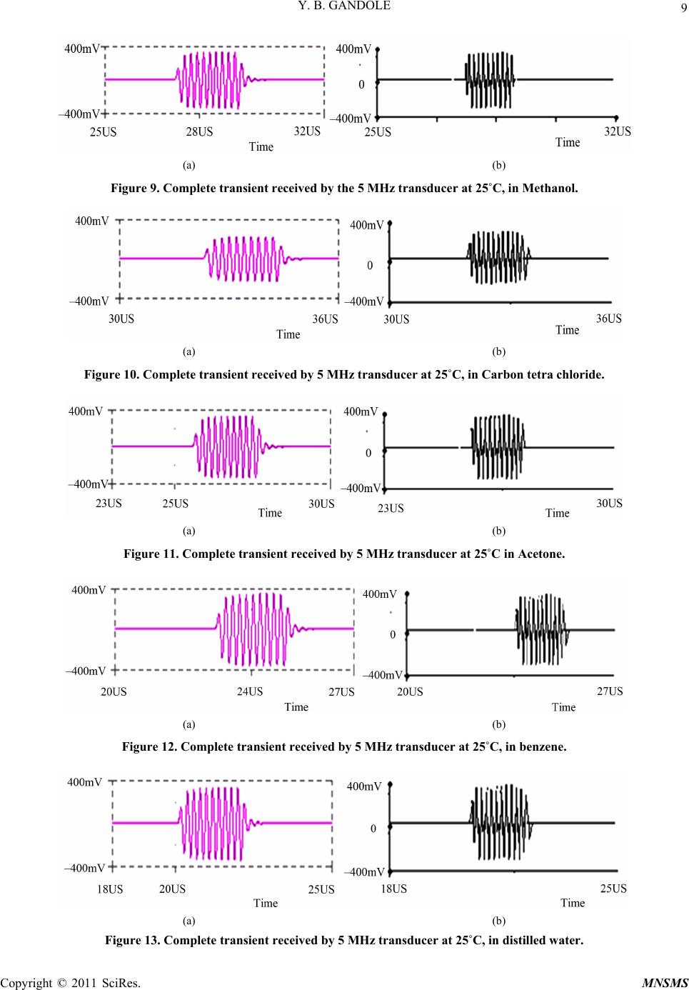
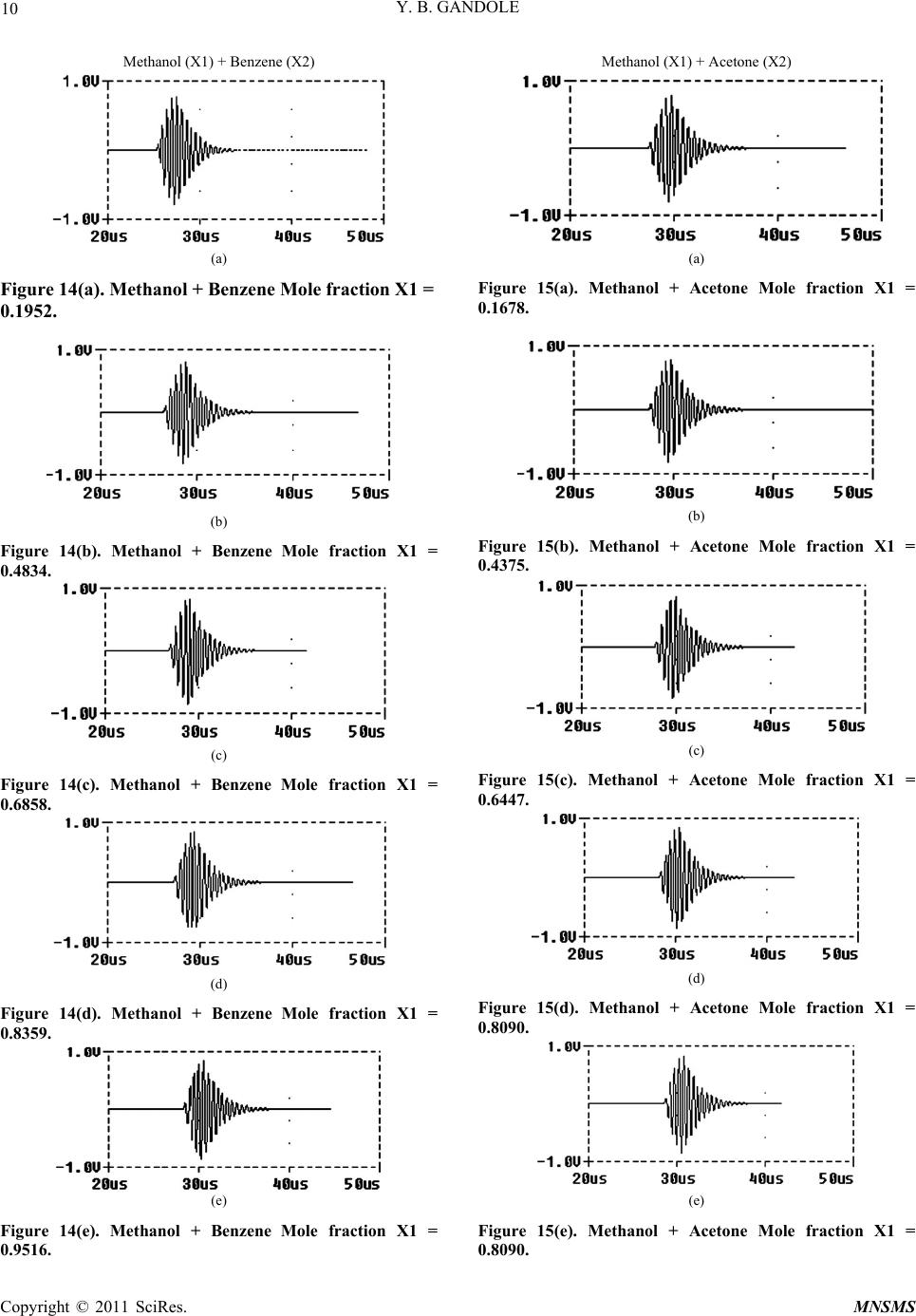
presented. The received signal from the simulation is
compared to that of an actual measurement in the time
domain. The comparison of simulated, experimental data
clearly shows that temperature and frequency dependen-
cies of parameters of relevance to acoustic wave propa-
gation can be modeled. The feasibility has been demon-
strated in an ultrasound transducer setup for material
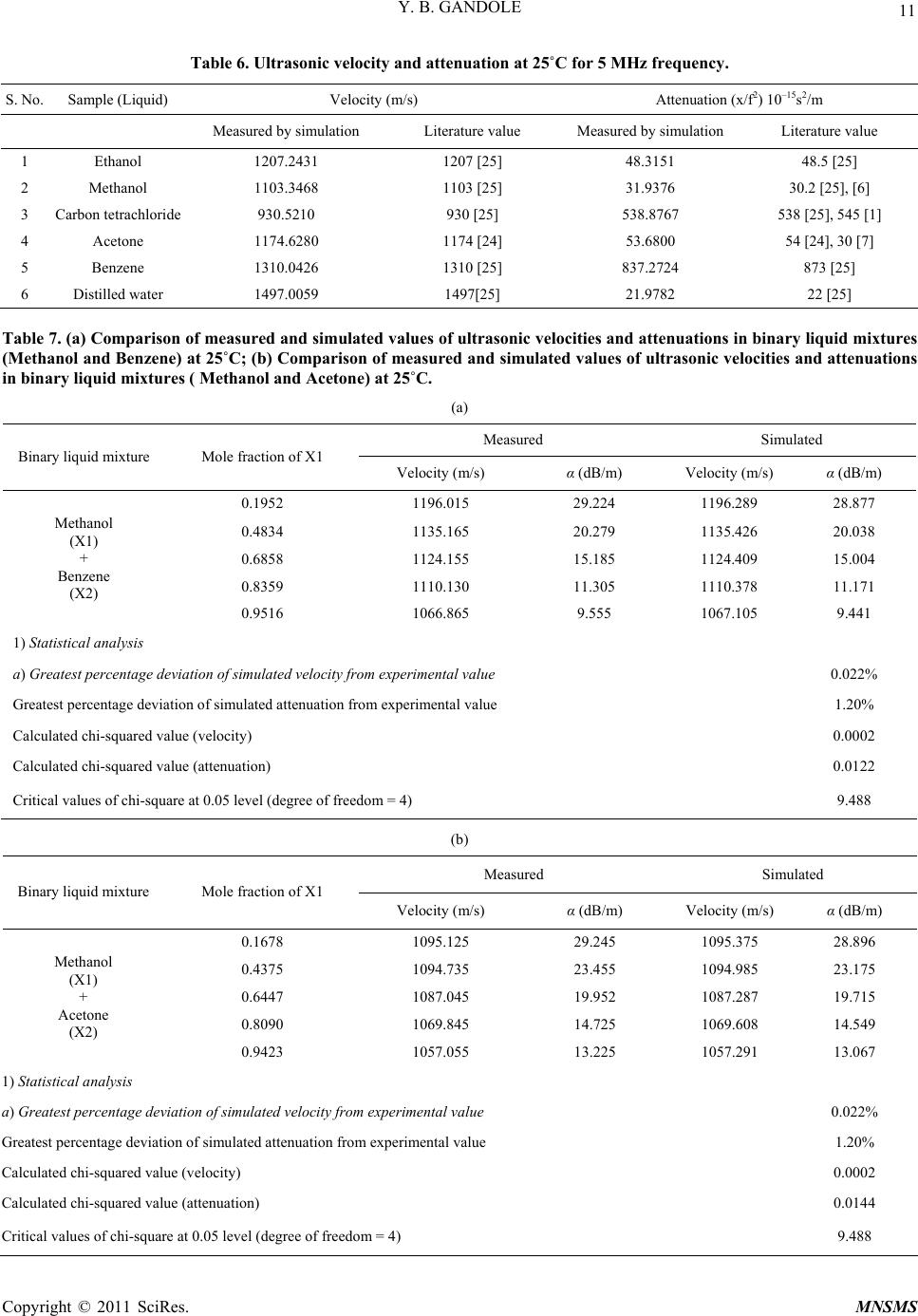
property investigations. Comparisons were made for at-
tenuation and velocity of sound for ethanol, methanol,
carbon tetrachloride, acetone, benzene and distilled water.
For these materials, the agreement is good. The simula-
tion tool therefore provides a way to predict the received
signal before anything is built. Furthermore, the use of an
ultrasonic simulation package allows for the develop-
ment of the associated electronics to amplify and process
the received ultrasonic signals.
7. References
[1] A. A. Berdyev and B. Khemraev, Russian Journal of
Physical Chemistry, Vol. 41, 1976, p. 1490.
[2] A. D. Pierce, “An Introduction to Its Physic Principles
and Applications,” Woodburg, New York, 1989.
[3] A. Puttmer, P. Hauptmann, R. Lucklum, O. Krause and B.
Henning, “SPICE Model for Lossy Piezoceramic Trans-
ducers,” IEEE Transactions on Ultrasonics, Ferroelec-
trics and Frequency Control, Vol. 44, No. 1, 1997, pp.
60-66. doi:10.1109/58.585191
[4] G. Benny, G. Hayward and R. Chapman, “Beam Profile
Measurements and Simulations for Ultrasonic Transduc-
ers Operating in Air,” Journal of the Acoustical Society of
America, Vol. 107, No. 4, 2000, pp. 2089-2100.
doi:10.1121/1.428491
[5] D. Berlincourt, H. A. Krueger and C. Near, “Important
Properties of Morgan Electroceramics,” Morgan Electro-
ceramics, Technical Publication, TP-226, 2001.
[6] D. E. Gray, “American Institute of Physics Handbook,”
3rd Edition, Mc Graw-Hill, New York, 1972.
[7] D. F. Evans, J. Thomas, J. A. Nadas and M. A. Matesich,
Journal of Physics and Chemistry, Vol. 75, No. 11, 1971,
pp. 1714-1722. doi:10.1021/j100906a013
[8] D. K. Cheng, “Field and Wave Electromagnetics,” 2nd
Edition, Addison-Wesley, Reading, 1989.
[9] G. S. Kino, “Acoustic Waves: Devices, Imaging and
Analog Signal Processing,” Prentice-Hall, Englewood
Cliffs, 1988.
[10] L. E. Kinsler, A. R. Frey, A. B. Coppens and J. V. Sand-
ers, “Fundamentals of Acoustics,” 3rd Edition, Wiley,
New York, 1982.
[11] M. Redwood, “Transient Performance of a Piezoelectric-
transducer,” Journal of the Acoustical Society of America,
Vol. 33, 1961, pp. 527-536. doi:10.1121/1.1908709
[12] M. G. S. Ali, “Analysis of Broadband Piezoelectric
Transducers by Discreet Time Model,” Egyptian Journal
of Solids, Vol. 23, 2000, pp. 287-295.
[13] M. Hirsekorn, P. P. Delsanto, N. K. Batra and P. Matic,
“Modellling and Simulation of Acoustic Wave Propagation
in Locally Resonant Sonic Materials,” Ultrasonics, Vol.
42, No. 1-9, 2004, pp. 231-235.
doi:10.1016/j.ultras.2004.01.014
[14] J. Millman and C. Halkias, “Integrated Electronics,”
McHill Ltd., Tokyo, 1972, p. 560.
[15] M. H. Rashid, “SPICE for Circuits and Electronics Using
PSPICE,” 2nd Edition, Printice Hall of India Pvt, Ltd.,
New Delhi, 2002.
[16] R. Krimholtz, D. A. Leedom and G. L. Matthei, “New
Equivalent Circuits for Elementary Piezoelectric Trans-
ducers,” Electronics Letters, Vol. 6, 1970, pp. 398-399.
doi:10.1049/el:19700280
[17] S. A. Morris and C. G. Hutchens, “Implementation of
Mason’s Model on Circuit Analysis Programs,” IEEE
Transactions on Ultrasonics, Ferroelectrics and Fre-
quency Control, Vol. 33, 1986, pp. 295-298.
[18] Y. B. Gandole, S. P. Yawale and S. S. Yawale, “Simpli-
fied Instrumentation for Ultrasonic Measurements,” Elec-
tronic Technical Acoustics, Vol. 35, 2005.
[19] J. L. San Emeterio, A. Ramos, P. T. sanz, A. Ruiz and A.
Azbaid, “Modeling NDT Piezoelectric Ultrasonic Trans-
mitter,” Ultrasonics, Vol. 42, No. 1-9, 2004, pp. 277-281.
doi:10.1016/j.ultras.2004.01.021
[20] J. P. Sferruzza, F. Chavrier, A. Birer and D. Cathignol,
“Numerical Simulation of the Electro-Acoustical Re-
sponse of a Transducer Excited by a Time-Varying Elec-
trical Circuit,” IEEE Transactions on Ultrasonics, Ferro-
electrics and Frequency Control, Vol. 49, No. 2, 2002, pp.
177-183.
[21] S. H. Lee, “Shear Viscosity of Benzene, Toluene, and
p-Xylene by Non-Equilibrium Molecular Dynamics
Simulations,” Bulletin of the Korean Chemical Society,
Vol. 25, No. 2, 2004, pp. 321-324.
doi:10.5012/bkcs.2004.25.2.321
[22] W. M. Leach, “Controlled-Source Analogous Circuits
and SPICE Models for Piezoelectric Transducers,” IEEE
Transactions on Ultrasonics, Ferroelectrics and Fre-
quency Control, Vol. 41, 1994, pp. 60-66.
[23] W. P. Mason, “Electromechanical Transducers and Wave
Filters,” Van Nostrand, New York, 1942.
[24] W. Schaaff, “Numerical Data and Functional Relational-
ships in Science and Technology,” In: K. H. Hellwege
and A. M. Hellweg, Eds., New Seris Group II: Atomic
and Molecular Physics, Vol. 5: Molecular Acoustics,
Springer-Verlag, Berlin, 1967.
[25] Weast, C. Robert, “Handbook of Chemistry and Physics,”
45th Edition, Chemical Rubber Co., Cleveland Ohio,

13 Y. B. GANDOLE
1964, p. E-28.
[26] X. Q. Bao, Y. Bar-Cohen, Z. Chang, B. P. Dolgin, S.
Sherrit, D. S. Pal, S. Du and T. Peterson, “Modeling and
Computer Simulation of Ultrasonic/Sonic Driller/Corer
(USDC),” IEEE Transactions on Ultrasonics, Ferroelec-
trics and Frequency Control, Vol. 50, No. 9, 2003, pp.
1147-1160.