 Open Journal of Com p osi t e M at e ri al s, 2011, 1, 19-37 doi:10.4236/ojcm.2011.11003 Published Online October 2011 (http://www.SciRP.org/journal/ojcm) Copyright © 2011 SciRes. OJCM Multi-Scale Modeling of Metal-Composite Interfaces in Titanium-Graphite Fiber Metal Laminates Part I: Molecular Scale Jacob M. Hundley1*, H. Thomas Hahn2, Jenn-Ming Yang3, Andrew B. Facciano4 1Mechanical and Aerospace Engineering Department, Multifunctional Composites Lab (MCL), University of California Los Angeles, Los Angeles, USA 2Raytheon Distinguished Professor Emeritus, Mechani cal and Aerospace Engineering Department, University of California Los Angeles, Los Angeles, USA 3Materials Sci ence and Engi n ee ri ng De p art me nt, University of California Los Angeles, Los Angeles, USA 4Raytheon Missile Systems, SM3 Syste m s E ngineering 1151, Tucson, USA E-mail: *jhundley@ucla.edu Received August 12, 2011; revised September 16, 2011; accept ed September 25, 2011 Abstract This study presents the first stage of a multi-scale numerical framework designed to predict the non-linear constitutive behavior of metal-composite interfaces in titanium-graphite fiber metal laminates. Scanning electron microscopy and x-ray diffraction techniques are used to characterize the baseline physical and chemical state of the interface. The physics of adhesion between the metal and polymer matrix composite components are then evaluated on the atomistic scale using molecular dynamics simulations. Interfacial me- chanical properties are subsequently derived from these simulations using classical mechanics and thermo- dynamics. These molecular-level property predictions are used in a companion study to parameterize a con- tinuum-level finite element model of the interface by means of a traction-separation constitutive law. Exten- sion of the proposed approach to other dissimilar metal- or metal oxide-polymer interfaces is also discussed. Keywords: Fiber Metal Laminates (FML), Titanium-Graphite (TiGr), Molecular Dynamics (MD), Adhesion 1. Introduction Fiber metal laminates (FMLs) are a unique class of structural materials that combine traditional fiber-reinfor- ced polymer matrix composite (PMC) laminae with thin, adhesively bonded metal layers. In these FML systems, the metal reinforcement layer(s) can be added to the PMC structure either internally or externally, provided that the fiber-reinforced polymer and metal layers are bonded together during the composite consolidation process. Consequently, the resultant structure is globally homogeneous but locally heterogeneous, with distinct material phases evident by visual inspection, Figure 1. First developed at Delft University of Technology in the late 1970s, commercially available examples of fiber metal laminates include GLARE (glass fiber-reinforced aluminum laminates) and ARALL (aramid fiber- reinforced aluminum laminates) [1]. Recently, a novel FML variant has been developed combining carbon fi- ber-reinforced polymer matrix composites with adhe- sively bonded titanium layers [2]. These FMLs are the focus of the present study and are commonly referred to as titanium-graphite (TiGr) or hybrid titanium co mposite laminates (HTCL). TiGr FMLs represent an intriguing material system as they possess increased stiffness and strength in comparison to ARALL and GLARE. They can also be utilized in elevated temperature applications, provided that the polymer matrix material has sufficient thermal degradation resistance. The primary advantage of all fiber metal laminate variants is their ‘best of both worlds’ design, in which the beneficial properties of the individual metal and PMC constituents are combined into a single structure with customizable material properties [3]. In essence, fiber metal laminates utilize the syn ergistic enhancement of structural properties achieved by combining two ma-  J. M. HUNDLEY ET AL. 20 Figure 1. Schematic illustration of the components in a fiber metal laminate. terials (metals and PMCs) with counterbalanced strengths and weaknesses. Because the limitations of each constituent are effectively offset, FMLs can be used in applications which are typically considered ill-suited for either metals or polymer matrix composites, such as impact-critical or mechanically fastened structures [4-9]. For each of these scenarios, it is important to note that the amount of improvement offered by an FML over a traditional metal or composite structure is heavily de- pendent upon the state of the interface between the metal and PMC constituents [10]. For instance, in impact- critical structures the formation and propagation of a delamination zone between the metal and PMC layers reduces the overall damage tolerance and impact energy dissipation potential of the FML. In addition to this loss of damage tolerance, interfacial delamination resulting from impact has also been shown to significantly reduce the residual static and fatigue strength of the FML [11]. For mechanically fastened fiber metal laminate structures, interfacial delamination prevents th e metal reinforcement layers from alleviating the high stress concentration in the region surrounding the fastener. As such, the result- ing delaminated FML is highly notch sensitive and will fail at lower than expected joint loads [6]. It is, therefore, highly desirable to form and maintain a strong inter- laminar bond between the polymer matrix adhesive and the metal adhered in any FML system so that these components do not delaminate. The importance of the metal-composite interface with respect to the structural performance of any FML v ariant underscores the evident need for accurate predictive models of interfacial mechanical behavior. However, it should be noted that prediction of adhesion between any two dissimilar components at a common interface is one of the most challenging and complex problems in the realm of materials modeling. The inherent difficulty is primarily due to the multiple length scales and damage modes associated with interfacial debonding and failure. For FMLs, this complexity means that any metal- composite interfacial model must be multi-scale. It must incorporate molecular-level considerations arising from separation of the interface, as well as continuum-level damage and failure phenomena due to microcracking and fracture of the polymer matrix. The present analysis is concerned with the development of one such multi-scale interface model, specifically applied and validated for use with TiGr FMLs. Establishment of the molecu- lar-level simulation methodology and physical/chemical characterization of the metal-composite interface are described herein. The coupled continuum-level modeling approach and experimental validation of the multi-scale framework will be covered in detail in a companion study. 2. Tigr Processing and Interfacial Characterization 2.1. Titanium Surface Treatment In the fabrication of any fiber metal laminate system, formation of a strong interlaminar bond between the metal and polymer matrix composite layers of the FML is of the utmost importance. In the specific case of tita- nium-graphite FMLs, the metal-composite interface must also be capable of withstanding the large residual ther- mal stress state that is introduced during the FML con- Co pyright © 2011 SciRes. OJCM  J. M. HUNDLEY ET AL.21 solidation process. These residual stresses are caused by a sizable mismatch in the thermal expansion coefficients of adjacent titanium and PMC layers. In the as-received state, the interlaminar bond strength between the un- modified titanium and the polymer matrix is typically not sufficient to endure these residual thermal stresses, re- sulting in delaminatio n after completion of the cure cycle [12,13]. Thus, in order to increase the strength and reli- ability of the TiGr metal-composite interface, a recently proposed chromium-free sequential acid-base titanium surface treatment procedure was employed [14]. It should be noted that the surface treatment process vari- ables were slightly modified to adapt the process to the un-alloyed commercially pure (CP) titanium used in this study. The ability of this chromium-free chemical treatment process to physically alter the CP titanium surface is evident from comparison of Figure 2 and Figure 3, which show scanning electron microscope (SEM) images obtained using a JEOL 6700F field emission SEM for pre- and post-treated CP titanium foil. In Figure 2, the non-uniform preexisting surface oxide layer is preferen- tially aligned with the rolling direction of the foil, and only provides partial surface coverage. After completion of the surface treatment process, this preferential orienta- tion disappears and full surface coverage is achieved, as shown in Figure 3. Coverage of the CP titanium surface with a protective titanium dioxide (TiO2) layer is the primary basis for enhanced interlaminar bond strength obtained using this sequential acid-base surface treat- ment method [14]. Additionally, comparison of the as-received and surface treated titanium foil surfaces shown respectively in Figure 2 and Figure 3 indicates that the surface treated titaniu m possesses a much higher degree of surface roughness in comparison the as-re- ceived titanium. This increased surface roughness also contributes to the interlaminar bond strength improve- ment, since it represents a larger active surface area be- tween the polymer matrix adhesive and the titanium ad- hered. 2.2. Characterization of the Titanium Dioxide Surface Layer In the preceding discussion, it was assumed a priori that changes in the CP titanium surface morphology, exhib- ited in Figure 3, were attributable to the formation of a titanium dioxide layer on the surface of the foil. How- ever, it should be noted that such chemical changes can- not be determined through visual inspection alone (i.e. scanning electron or optical microscopy). Therefore, elemental characterization of the surface treated CP tita- nium foil was required to confirm an increase in oxygen content at the foil surface, consistent with the presence of a titanium dioxide layer. To quantify the chemical com- position of the material, a total of four 6.35 mm by 6.35 mm samples were cut from random locations in two sur- face treated and as-received titanium foil sheets. These samples were then analyzed using an energy dispersive X-ray (EDX) spectroscopy system attached to the JEOL scanning electron microscope. Figure 4 provides the representative EDX spectra for both the as-received and surface treated titanium foil, with each spectrum normal- ized and offset for clarity. From this figure and the ele- mental reference peak energy values listed in Table 1, it is evident that the surface treated titanium foil exhibits a clear peak corresponding to the oxygen Kα x-ray radia- tion energy (0.525 keV). Comparatively, the as-received titanium foil contains only Ti peaks (Ti Kα, Ti Kβ, and Ti LI), which is expected for an unalloyed and theoreti- cally uncontaminated material. From the EDX measure- ments, the oxygen Kα peak obtained for the surface treated samples indicates the presence of the previously assumed oxide layer on the titanium foil surface. While the comparative EDX spectra of Figure 4 are ideal for determining the elemental composition of a given material, they provide no information as to its crystalline structure. This distinction is particularly im- portant for titanium dioxide, since it naturally occurs in three distinct polymorphs; rutile, anatase, and brookite. Of these three, rutile, represents the most common phase [15]. Given that the positions of the titanium and oxygen atoms within the TiO2 lattice and the atomic packing density are both functions of the crystallin e phase, struc- tural characterization is essential for accurate molecu- lar-level modeling. In order to determine the crystalline structure of the titanium dioxide surface layer, a total of four 5.08 cm by 2.54 cm samples were cut from random locations in the same as-received and surface treated titanium foil sheets. These samples were subsequently analyzed using a Panalytical X’Pert Pro X-ray powder diffraction (XRD) system. X-ray intensity was measured for each sample at room temperature over a detector an- gle ( 2 ) range of 25˚ to 45˚ using a Cu-target X-ray tube with wavelength of 1.542 Å, operated at 1800 watts. Normalized X-ray diffraction patterns obtained using these settings are shown in Figure 5 and Figure 6 for the as-received and surface treated CP titanium samples, respectively. As with the EDX spectra discussed previ- ously, there is an eviden t distinction between the diffrac- tion patterns of the as-received and surface treated tita- nium foil. As expected, detector angles corresponding to the X-ray intensity peaks of Fig ure 5 show go od co rr ela- tion with the powder diffraction file (PDF) reference peak locations for unalloyed α-phase titanium, with the highest intensity peaks occurring at detector angles of Copyright © 2011 SciRes. OJCM  J. M. HUNDLEY ET AL. 22 Figure 2. Scanning electron micrograph (2000× magnification) of the as-received CP titanium foil surface showing preexist- ing oxide layer pref erentially align ed w it h foil rolling direction (length of the page). Figure 3. Scanning electron micrograph (2000× magnification) of the treated CP titanium foil surface. 38.3˚ and 40.2˚ [16]. The detector angles which corre- spond to observed peaks in the as-received samples and correspond to PDF reference peak locations for α-phase titanium are provided in Table 2. In comparison, inves- tigation of the surface treated titanium XRD pattern of Figure 6 shows the same α-phase Ti peaks, although at reduced relative intensities and slightly shifted to lower detector angles. Additionally, a series of peaks attribut- able to the titanium dioxide surface layer are also evident in the treated CP titanium samples. In Figure 6, the highest intensity peak now resides at a detector angle of 27.4˚. Comparison of this XRD pattern with the PDF Co pyright © 2011 SciRes. OJCM  J. M. HUNDLEY ET AL. 23 Figure 4. EDX spectra for as-received (bottom) and surface treated (top) CP titanium foil with elemental reference peak in- dicators. Table 1. Measured EDX energy values for as-received and surface treated CP Ti. X-Ray Energy (keV) EDX Spectrum Type Ti L O Kα Ti Kα Ti Kβ As-Received CP Titanium 0.39 - 4.52 4.94 Surface Treated CP Titanium 0.43 0.52 4.52 4.93 Reference Peak Energies 0.40 0.53 4.51 4.93 Table 2. Measured XRD peak detector angles for as-received surface treated CP Ti. Peak Locations - Detector Ang le (2θ) Spectrum Type Peak 1 Peak 2 Peak 3 Peak 4 Peak 5 Peak 6 Peak 7 Peak 8 As-Received CP Titanium - 35.08 - 38.34 - 40.15 - - Surface Treated CP Titanium 27.44 34.90 36.07 37.72 39.18 39.79 41.25 44.02 PDF 44-1294 (α-Ti) - 35.09 - 38.42 - 40.17 - - PDF 21-1276 (Rutile TiO2) 27.41 - 36.03 - 39.21 - 41.23 44.07 Co pyright © 2011 SciRes. OJCM  J. M. HUNDLEY ET AL. Copyright © 2011 SciRes. OJCM 24 Figure 5. XRD pattern for as-received CP titanium with reference peak locations. Figure 6. XRD pattern for surface treated CP titanium with reference peak locations.  J. M. HUNDLEY ET AL. 25 references for titanium dioxide polymorphs indicates that the titanium dioxide surface layer is in the rutile crystal- line phase, as indicated by the peak location detector angles provided in Table 2 [17]. 2.3. Titanium-Graphite Fiber Metal Laminate Fabrication Following characterization of the titanium dioxide sur- face layer, a set of two 10.16 cm by 15.24 cm tita- nium-graphite fiber metal laminate panels were fabri- cated, each with an identical [0/45/Ti/-45/90]s stacking sequence. A [0/45/Ti/-45/90]s layup was chosen since it had been shown previously to provide the optimum spe- cific properties (property ratio with respect to density) for mechanically fastened titanium-graphite fiber metal laminate joints [18]. The polymer matrix composite lay- ers of these TiGr FML panels consisted of unidirectional carbon fiber-reinforced toughened epoxy prepreg tape (CYCOM 977-3/IM7), obtained from Cytec Industries. Panel consolidation was performed in a 2 ft by 5 ft Thermal Equipment autoclave, according to the prepreg manufacturer’s suggested cure cycle, with a maximum temperature of 177˚C and a sustained application pres- sure of 0.586 MPa [19]. After completion of the panel cure cycle, an optical microscopy investigation of each TiGr panel cross-section indicated that the panels were well consolidated, with the metal-composite interfaces free of discontinuities, as shown in Figure 7. In addition, enhanced magnification SEM images obtained at the metal-polymer interfaces revealed excellent continuity between the dissimilar materials down to the mi- cron-scale, as evidenced by Figure 8. In this figure, the bright line at the boundary between the titanium rein- forcement and the epoxy matrix corresponds to the tita- nium dioxide surface layer. Since titanium dioxide is highly resistive, particularly with respect to the titanium substrate and the IM7 carbon fibers, charging effects from the SEM electron beam make the TiO2 layer highly visible. 3. Simulation of the Interfacial Molecular Structure 3.1. Computational Methods for Molecular Simulation In order to numerically reproduce the bonded metal- composite interface shown in Figure 8, the molecular basis for adhesion between the titanium dioxide and ep- oxy constituents was evaluated using molecular dynam- ics (MD) simulations. Molecular dynamics is essentially a numerical solution to a general n-body problem, in Figure 7. Optical micrograph (100× magnification) of a [0/45/Ti/-45/90]s TiGr FML cross-section. which the interaction physics between neighboring bod- ies (atoms) are approximated using a pre-defined force- field or potential energy expression. Given that these simulations are classical in nature, quantum mechanics Co pyright © 2011 SciRes. OJCM  J. M. HUNDLEY ET AL. 26 Figure 8. Scanning electron micrograph (3000 × magnification) of the titanium/45° composite interface in a [0/45/Ti/-45/90]s TiGr FML. effects or other related phenomena are not considered. In this analysis, commercially available MD simulation software (Materials Studio) from Accelrys Inc. was used to generate molecular-level structure and property pre- dictions for metal-composite interfaces in TiGr FMLs. The Materials Studio software suite contains a version of the condensed-phase optimized molecular potentials for atomistic simulation studies (COMPASS) forcefield, an ab initio forcefield which has been parameterized and validated using condensed-phase properties [20]. In the COMPASS forcefield, the general relationship between any two atoms in the simulation can be defined by the following functional fo rm of the potential energy expr es- sion, which is a linear combination of all possible bonded (B), cross-term (CT), and non-bonded (NB) in- teractions [20]: totalB CTNB UUUU (1) Specific forms of the bonded and cross-term interac- tions in the above potential energy expression can be obtained from literature. However, since this analysis is primarily concerned with the non-bonded interactions between atoms that describe the behavior of physisorbed interfaces, the functional form of UNB is provided in Equation (2): 96 i jijij NB ij ij ij ij qqA B Ur rr r (2) In the above equation, the non-bonded interaction en- ergy component consists of electrostatic and Leo- nard-Jones potential terms, where rij is the spatial posi- tion vector between the two atoms and qi and qj are the atomic charges. Additionally, Aij, Bij, and ε are mate- rial-dependant constants, which must be determined for any unique interaction between two atoms in the simula- tion. A major advantage of a commercially available software package, such as Materials Studio, is that the material constants necessary in the evaluation of Equa- tion (2) have been previously determined for a variety of atomic configurations. Therefore, no additional parame- terization of the COMPASS forcefield is required. 3.2. Molecular Modeling of the Metal-Composite Interface To simulate the mechanics of adhesion at the titanium dioxide-epoxy interfaces in a TiGr FML, the COMPASS forcefield and the functional forms of the system’s total potential energy and the non-bond interaction energy provided in Equations (1)-(2) were used in a series of MD simulations to construct represen tative models of the molecular-level interfacial structure. Formation of a tita- nium dioxide simulation cell was the first step in the construction of this model, requiring knowledge of the TiO2 lattice parameters and atomic positions, as well as the exposed crystalline surface. From the X-ray diffrac- tion pattern of Figure 6, it was previously determined that the CP titanium reinforcement layers in the TiGr Co pyright © 2011 SciRes. OJCM  J. M. HUNDLEY ET AL.27 FMLs possessed a rutile-phase titanium dioxide surface structure. The unit cell of this particular TiO2 polymorph is tetragonal, with a TiO6 octahedron forming the basic structural unit of the crystal. The lattice parameters and atomic coordinates necessary for molecular modeling of rutile TiO2 are well established in the literature, and are listed in Table 3 [22]. However, it should be noted that the exterior faces of the unit cell formed by these lattice parameters do not necessarily correspond to the exposed TiO2 crystallographic plane at the surface of the CP tita- nium reinforcement. In rutile TiO2, the predominately exposed crystalline cleave plane is the (110) face, and thus all titanium dioxide surface models presented in this study utilize TiO2 crystals terminated with the (110) plane [23]. Because the dimensions of a single TiO2 unit cell are much too small to produce physically relevant results, the simulation cell surface area (As) was in- creased by extending the crystal in each of the in-plane directions, as illustrated in Figure 9. This TiO 2 supercell was approximately tetragonal with dimensions of A=20.71 Å, B=19.47 Å, and C=14.94 Å. Prior to layer- ing the polymer molecules on top of this TiO2 supercell, a minimization of the sup ercell total p oten tial en ergy was performed using the COMPASS forcefield to obtain the equilibrium configuration of the exposed surface. As expected, the positions of all atoms in the TiO2 supercell did not significantly change following energy minimiza- tion, confirming the accuracy of the lattice parameters and atomic coordinates provided in Table 3. After building the titanium dioxide surface model, the interface between the metal and composite constituents in a TiGr FML was replicated at the molecular-level by layering a cross-linked epoxy structure on top of the en- ergy minimized TiO2 surface. Exclusion of the reinforc- ing fibers from the molecular-level interface model is a reasonable assumption, since SEM investigation showed that the carbon fiber-titanium separation distance was several orders of magnitude larger than the MD unit cell. It should also be noted that the stipulation of a cross-linked epoxy layer complicated the analysis somewhat, since the number and location of these cross-links was not known a priori. Therefore, it was first necessary to model the transformation of the linear epoxy molecules into a highly networked structure be- fore analyzing the resultant interface. Given that the be- havior of the epoxy resin near the interface will, in gen- eral, deviate from the behavior of the bulk epoxy, the MD cross-linking simulations were performed in the presence of the TiO2 surface. Although the actual for- mulation of the epoxy resin (CYCOM 977-3) is proprie- tary, it is widely assumed that this material is a tetragly- cidyl methylene dianiline (TGMDA) and dia- mino-diphenyl sulfone (DDS) blend, where the chemical Figure 9. Titanium dioxide unit cell and supercell configurations used for molecular simulation. Table 3. Lattice parameters and symmetry atomic coordinates for rutile TiO2 [22]. TiO2 Lattice Quantity a b c Lattice Parameters (Å) 0.4595 0.4595 0.2959 Ti Atomic Position (Fractional Coordinates) 0.0000 0.0000 0.0000 O Atomic Position (Fractional Coordinates) 0.3048 0.3048 0.0000 Copyright © 2011 SciRes. OJCM  J. M. HUNDLEY ET AL. 28 structures and molecular models for each linear epoxy constituent are shown in Figure 10 [24]. The individual epoxy constituents presented in Figure 10 were then energy-minimized and a total of eight distinct amorphous polymer cells were created, containing 74.5% TGMDA to 25.5% DDS by weight. Due to the highly unstructured nature of the liquid resin, these eight independent epoxy configurations were required to effectively ‘average out’ configuration-space effects. The planar dimensions of the amorphous epoxy cells were set equal to the lattice pa- rameters of the TiO2 surface (A=20.71 Å and B=19.47 Å), with the cell height constrained by the liquid-state density of the epoxy resin (1.1 6 g/cm3), determined from the manufacturer’s datasheet [19]. Each of the eight in- dependent configurations were then layered on top of the titanium dioxide surface and a 20 Å vacuum spacer layer was added to the top of the simulation cells. Figure 11 provides two-dimensional views for two of the eight unique Figure 10. Epoxy resin monomer (TGMDA) and cross-linking agent (DDS) molecular structure. Figure 11. MD interface model for the TiO2-line a r ep o x y system. Co pyright © 2011 SciRes. OJCM  J. M. HUNDLEY ET AL. 29 TiO2-linear epoxy interface configurations, each con- taining 1630 atoms. In the figure, it is important to note that periodic boundary conditions were applied for the in-plane directions (1- and 2-directions in Figure 11), but the presence of the vacuum spacer eliminated perio- dicity in the thickness (3) direction. In order to imitate formation of the networked epoxy structure, molecular dynamics cross-linking simulations were performed using the COMPASS forcefield with an isochoric-isobaric (NVT) canonical ensemble for each of the eight TiO2-linear epoxy simulation cells. In each case, the equilibrium configuration of the interface was deter- mined from 100 ps of dynamics time at 450K, which corresponded to the maximum applied temperature in the TiGr consolidation process [19]. The time step between successive dynamics increments was set at 1 fs, and a cutoff radius of 9.5 Å was used to determine the maxi- mum separation distance (rij) at which the non-bond en- ergy of Equation (2) was evaluated for each atom pair. Given that the potential energy of the TiO2 surface had previously been minimized, the positions of all atoms in the titanium dioxide supercell were fixed in place during the molecular dynamics run. A fixed surface assumption is valid since the TiO2 lattice parameters and atomic co- ordinates do not significantly vary (0.16%) over the temperature range of interest (298K to 450K) [22]. During the MD analysis, trajectories for all epoxy atoms in the model were stored at every 5 ps of simulation time, and were used to predict the resultin g cross-linked struc- ture according to the method outlined by Yarovsky and Evans [25]. In this method, cross-link formation in a thermosetting polymer is assumed to be directly related to the distance between the active sites of the linear polymer and cross-linking agent molecules. When these sites are within a specified interaction radius (6.0 Å in this study), cross-linking will occur. For a TGMDA/DDS system, the active sites for each molecule correspond to the epoxy (-C-O-C-) and amine (NH2) functional groups, as illustrated in Figure 12. Replication of this cross- linking process was performed by calculating the posi- tion of each active epoxy site from the MD trajectories and applying a nearest neighbor search algorithm to identify the corresponding amine site in closest prox- imity. If the distance between these two groups was less than or equal to the interaction radius, then the corre- sponding TGMDA and DDS molecules were connected in the MD simulation cell according to Figure 12. Ap- plication of this method to all eight TiO2-linear epoxy interface models resulted in an average cross-link effi- ciency of 83.9% after 100 ps of dynamics time. It is important to point out that the geometric ap- proximation of an essentially chemical process was ne- cessitated by the classical nature of molecular dynamics simulations. Because MD analyses are based upon nu- merical solution of the Newtonian equations of motion, charge transfer phenomena associated with the formation and breakage of chemical bonds cannot be explicitly modeled using MD techniques without the inclusion of quantum mechanics effects. Given that quantum calcula- tions for a system containing thousands of atoms become prohibitively exp ensive from a computational standpo int, the above geometric method represents the best predic- tive strategy for obtaining the fin al cross-linked configu- ration of the epoxy resin. Once the networked epoxy configurations had been formed, the final structure of each TiO2-epoxy interface was determined from a 200 ps molecular dynamics run at room temperature (298K). MD analyses of the cooled interface were, once again, performed using the COMPASS forcefield and an NVT ensemble. In this manner, a total of 300 ps of MD simu- lation time were used to determine the equilibrium state of each interface configuration; 100 ps for the linear ep- oxy at 450K and 200 ps for the cross-linked system at 298K. Figure 12. TGMDA/DDS epoxy cross-linking reaction. Co pyright © 2011 SciRes. OJCM  J. M. HUNDLEY ET AL. 30 4. Molecular-Level Interfacial Property Predictions 4.1. Interfacial Predictions across Multiple Length Scales The room temperature molecular configurations obtained for each of the eight simulation cells were then used to generate mechanical property predictions for the metal- composite interfaces in TiGr FMLs. In this analysis, the properties of interest are the transverse elastic constants (E33, G13, G23), ultimate normal and shear interfacial strength values (33 u ,13 u ,23 u ), corresponding strains at failure (33 ,13 ,23 ), and fracture energies (33 U,13 U, 23 U). However, it should be noted that only three of these component groups are independent, due to the in- tegral relationship between fracture energy and the stress-strain curves in each of the normal and shear modes. In this analysis, strain at failure was chosen as the interfacial dependent variable set, since its resolution from MD simulations contains the greatest ambiguity. To determine the remaining independent interfacial vari- ables, a series of calculations were performed using the predicted TiO 2-epoxy molecular structures obtained after 300 ps of MD simulation time. As will be discussed in the companion study, these MD-derived mechanical properties were integrated into a continuum-level finite element analysis via a traction-separation constitutive law. This propagation of molecular-level considerations up to the continuum-level is what gives the current model its multi-scale nature. 4.2. Calculation of Interfacial Fracture Energy Of these interfacial mechanical properties, fracture en- ergy is by far the most straightforward to determine from a molecular dynamics simulation. This is due to the analogous relationship between fracture energy and work of adhesion (Wad) for a bonded interface, in which ‘fail- ure’ is defined by separation of the heterogeneous inter- face into two distinct homogeneous components. For a chemical or mechanical bond between two materials, work of adhesion is the fundamental thermodynamic quantity which defines their dissociation at the molecu- lar-level. Experimental measurements of the work of adhesion are difficult to obtain and often overestimate the stability of the interface This is due to secondary en- ergy dissipation mechanisms in the sample which do not contribute to debonding (e.g. specimen relaxation and plasticity) [26]. Calculation of the work of adhesion in a molecular dynamics simulation is comparatively simple, since Wad is linearly dependent on the interaction energy (Uint) between the interface components: int S A ad I U W (3) Where (As)I represents the surface area of the interface with normal direction (I) and the interaction energy is defined by the total system energy and the surface free energies of each component of the interface (TiO2 and epoxy) as per the Dupré relationship [27]: 2 int TiO total epoxy UUUU (4) Computation of each term in Equation (4) in an MD analysis is straightforward because potential energy must be determined at each time step in order to solve the governing equations of motion. Therefore, for each of the eight TiO2-epoxy interface configurations, the work of adhesion at 298K was determined by calculating the potential energy o f the total system as well as that of the epoxy and titanium dioxide surfaces using the COM- PASS forcefield at the final MD time step (t = 200 ps). Using this method, the predicted work of adhesion for a TiO2-epoxy interface was found to be 1.12 ± 0.03 J/m2, where the uncertainty represents one standard deviation over all eight configurations. Because the surface area component of Wad in Equation (3) is always normal to the interface, it was assumed that the work of adhesion and fracture energy were mode-independent (i.e. Wad= 33 U, 13 U, 23 U). It should also be noted that while use of the final molecular trajectory (t = 200 ps) in the work of adhesion calculations was somewhat arbitrary, it did not greatly impact the predictio ns. This is due to the fact that the potential en ergy of each configur ation converg ed to an equilibrium state after approximately 7 ps of dy- namics time, as shown in Figure 13. 4.3. Calculation of Interfacial Normal and Shear Strength In addition to fracture energy, the interfacial strength in the shear and normal deformation modes was also calcu- lated from the equilibrium configurations of the TiO2-epoxy interface using energy considerations and the COMPASS forcefield [28]. From the potential en- ergy form in Equation (1), the inter- and intra-molecular forces (FI) acting on any atom in the MD simulation are related to the atomic total potential energy through the gradient operator: total II ij FUr (5) where summation is not applied for all lower case sub- scripts. While this equation is essential for the solution of the classical equations of motion in any MD analysis, it can also be used to calculate the tensile or shear stresses Co pyright © 2011 SciRes. OJCM 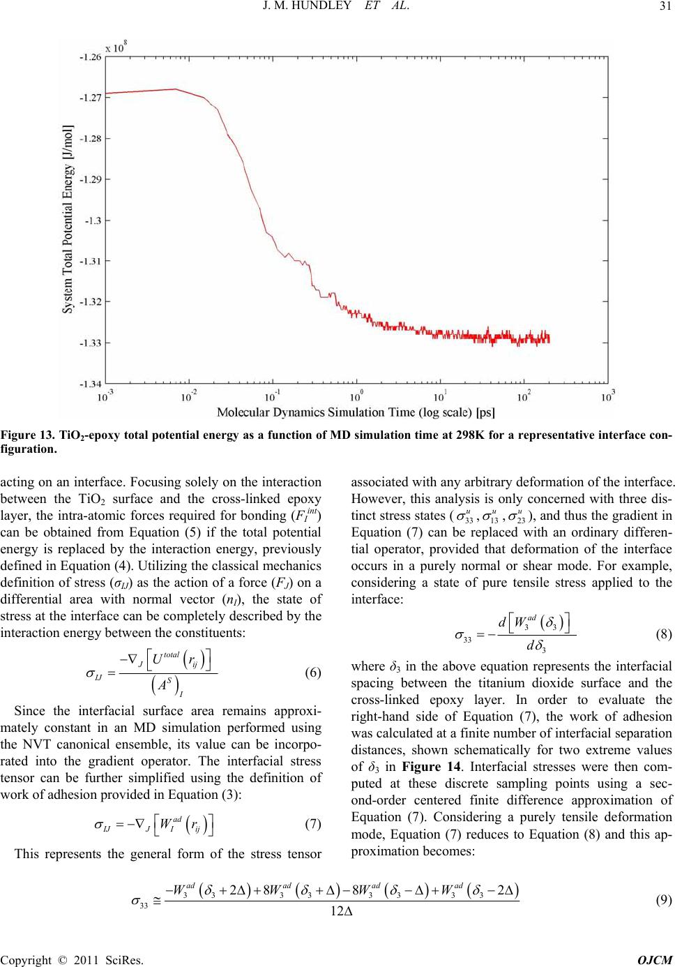 J. M. HUNDLEY ET AL. 31 Figure 13. TiO2-epoxy total potential energy as a function of MD simulation time at 298K for a representative interface con- figuration. acting on an interface. Focusing solely on the interaction between the TiO2 surface and the cross-linked epoxy layer, the intra-atomic forces required for bonding (FIint) can be obtained from Equation (5) if the total potential energy is replaced by the interaction energy, previously defined in Equation (4 ). Utilizing th e classical mechanics definition of stress (σIJ) as the action of a force (FJ) on a differential area with normal vector (nI), the state of stress at the interface can be completely described by the interaction energy between the constituents: total Jij IJ S I Ur A (6) Since the interfacial surface area remains approxi- mately constant in an MD simulation performed using the NVT canonical ensemble, its value can be incorpo- rated into the gradient operator. The interfacial stress tensor can be further simplified using the definition of work of adhesion provided in Equation (3): ad IJJ Iij Wr (7) This represents the general form of the stress tensor associated with any arbitrary deformation of the interface. However, this analysis is only concerned with three dis- tinct stress states (33 u ,13 u ,23 u ), and thus the gradient in Equation (7) can be replaced with an ordinary differen- tial operator, provided that deformation of the interface occurs in a purely normal or shear mode. For example, considering a state of pure tensile stress applied to the interface: 33 33 3 ad dW d (8) where δ3 in the above equation represents the interfacial spacing between the titanium dioxide surface and the cross-linked epoxy layer. In order to evaluate the right-hand side of Equation (7), the work of adhesion was calculated at a finite number of interfacial separation distances, shown schematically for two extreme values of δ3 in Figure 14. Interfacial stresses were then com- puted at these discrete sampling points using a sec- ond-order centered finite difference approximation of Equation (7). Considering a purely tensile deformation mode, Equation (7) reduces to Equation (8) and this ap- proximation becomes: 333333 33 33 28 82 12 adadad ad WWWW (9) Co pyright © 2011 SciRes. OJCM 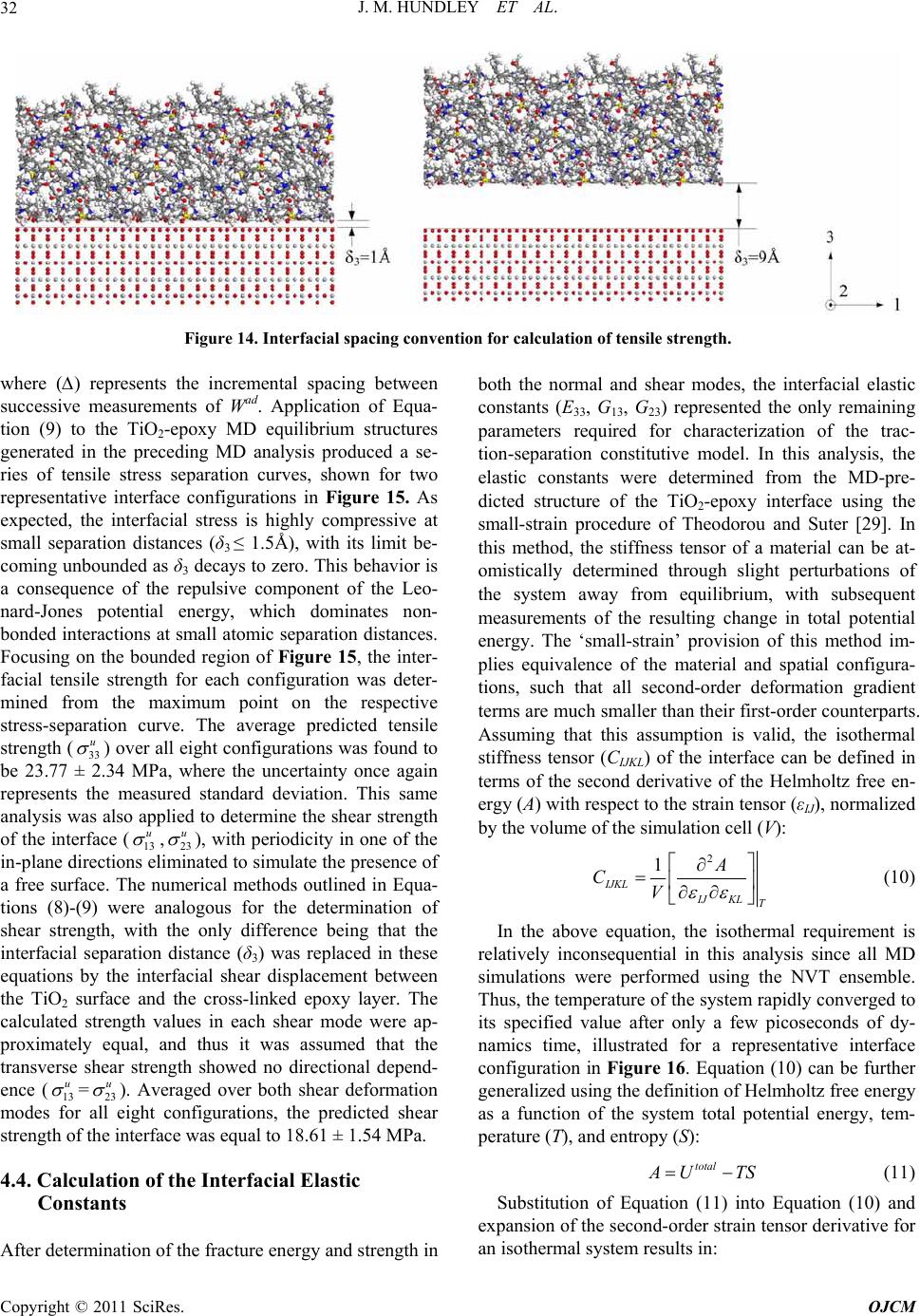 J. M. HUNDLEY ET AL. 32 Figure 14. Interfacial spacing convention for calculation of tensile strength. where (∆) represents the incremental spacing between successive measurements of Wad. Application of Equa- tion (9) to the TiO2-epoxy MD equilibrium structures generated in the preceding MD analysis produced a se- ries of tensile stress separation curves, shown for two representative interface configurations in Figure 15. As expected, the interfacial stress is highly compressive at small separation distances (δ3 ≤ 1.5Å), with its limit be- coming unbound ed as δ3 decays to zero. This behavior is a consequence of the repulsive component of the Leo- nard-Jones potential energy, which dominates non- bonded interaction s at small atomic separation distances. Focusing on the bounded region of Figure 15, the inter- facial tensile strength for each configuration was deter- mined from the maximum point on the respective stress-separation curve. The average predicted tensile strength (33 u ) over all eight config urations was found to be 23.77 ± 2.34 MPa, where the uncertainty once again represents the measured standard deviation. This same analysis was also applied to determine the shear strength of the interface (13 u ,23 u ), with periodicity in one of the in-plane directions eliminated to simulate the presence of a free surface. The numerical methods outlined in Equa- tions (8)-(9) were analogous for the determination of shear strength, with the only difference being that the interfacial separation distance (δ3) was replaced in these equations by the interfacial shear displacement between the TiO2 surface and the cross-linked epoxy layer. The calculated strength values in each shear mode were ap- proximately equal, and thus it was assumed that the transverse shear strength showed no directional depend- ence (13 u =23 u ). Averaged over both shear deformation modes for all eight configurations, the predicted shear strength of the interface was equal to 18.61 ± 1.54 MPa. 4.4. Calculation of the Interfacial Elastic Constants After determination of the fracture energy and strength in both the normal and shear modes, the interfacial elastic constants (E33, G13, G23) represented the only remaining parameters required for characterization of the trac- tion-separation constitutive model. In this analysis, the elastic constants were determined from the MD-pre- dicted structure of the TiO2-epoxy interface using the small-strain procedure of Theodorou and Suter [29]. In this method, the stiffness tensor of a material can be at- omistically determined through slight perturbations of the system away from equilibrium, with subsequent measurements of the resulting change in total potential energy. The ‘small-strain’ provision of this method im- plies equivalence of the material and spatial configura- tions, such that all second-order deformation gradient terms are much smaller than their first-order counterparts. Assuming that this assumption is valid, the isothermal stiffness tensor (CIJKL) of the interface can be defined in terms of the second derivative of the Helmholtz free en- ergy (A) with respect to the strain tensor (εIJ), normalized by the volume of the simulation cell (V): 2 1 IJKL IJKL T A CV (10) In the above equation, the isothermal requirement is relatively inconsequential in this analysis since all MD simulations were performed using the NVT ensemble. Thus, the temperature of the system rapidly converged to its specified value after only a few picoseconds of dy- namics time, illustrated for a representative interface configuration in Figure 16. Equation (10) can be further generalized using the definition of Helmholtz free energy as a function of the system total potential energy, tem- perature (T), and entropy (S): total UTS (11) Substitution of Equation (11) into Equation (10) and expansion of the second-order strain tensor derivative for an isothermal system results in: Copyright © 2011 SciRes. OJCM 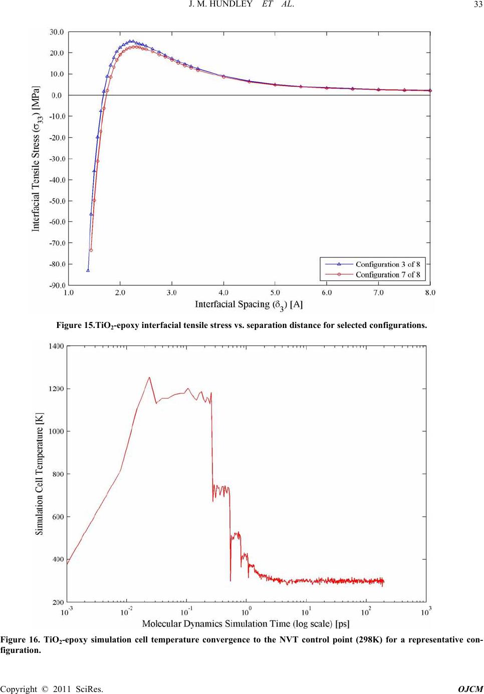 J. M. HUNDLEY ET AL. 33 Figure 15.TiO2-epoxy interfacial tensile stress vs. separation distance for selected configurations. Figure 16. TiO2-epoxy simulation cell temperature convergence to the NVT control point (298K) for a representative con- figuration. Co pyright © 2011 SciRes. OJCM 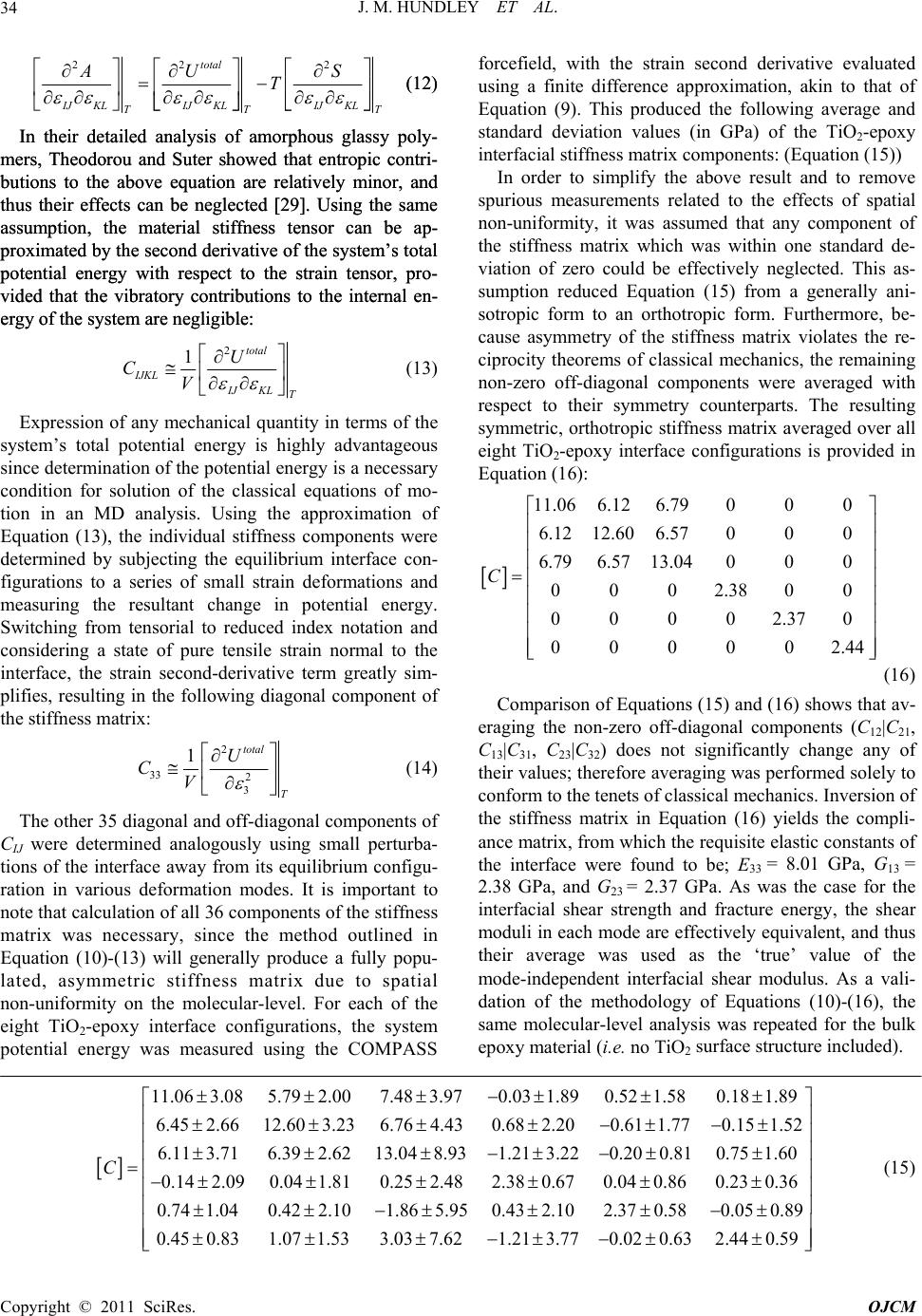 J. M. HUNDLEY ET AL. 34 22 2total IJ KLIJ KLIJ KL TT AU S T T (12) (12) In their detailed analysis of amorphous glassy poly- mers, Theodorou and Suter showed that entropic contri- butions to the above equation are relatively minor, and thus their effects can be neglected [29]. Using the same assumption, the material stiffness tensor can be ap- proximated by the second derivative of the system’s total potential energy with respect to the strain tensor, pro- vided that the vibratory contributions to the internal en- ergy of the system are negligible: In their detailed analysis of amorphous glassy poly- mers, Theodorou and Suter showed that entropic contri- butions to the above equation are relatively minor, and thus their effects can be neglected [29]. Using the same assumption, the material stiffness tensor can be ap- proximated by the second derivative of the system’s total potential energy with respect to the strain tensor, pro- vided that the vibratory contributions to the internal en- ergy of the system are negligible: 2 1total IJKL IJKL T U CV (13) Expression of any mechanical quantity in terms of the system’s total potential energy is highly advantageous since determination of the potential energy is a necessary condition for solution of the classical equations of mo- tion in an MD analysis. Using the approximation of Equation (13), the individual stiffness components were determined by subjecting the equilibrium interface con- figurations to a series of small strain deformations and measuring the resultant change in potential energy. Switching from tensorial to reduced index notation and considering a state of pure tensile strain normal to the interface, the strain second-derivative term greatly sim- plifies, resulting in the following diagonal component of the stiffness matrix: 2 33 2 3 1total T U CV (14) The other 35 diagonal and off-di agonal componen ts of CIJ were determined analogously using small perturba- tions of the interface away from its equilibrium configu- ration in various deformation modes. It is important to note that calculation of all 36 components of the stiffness matrix was necessary, since the method outlined in Equation (10)-(13) will generally produce a fully popu- lated, asymmetric stiffness matrix due to spatial non-uniformity on the molecular-level. For each of the eight TiO2-epoxy interface configurations, the system potential energy was measured using the COMPASS forcefield, with the strain second derivative evaluated using a finite difference approximation, akin to that of Equation (9). This produced the following average and standard deviation values (in GPa) of the TiO2-epoxy interfacial stiffness matrix components: (Equation (15)) In order to simplify the above result and to remove spurious measurements related to the effects of spatial non-uniformity, it was assumed that any component of the stiffness matrix which was within one standard de- viation of zero could be effectively neglected. This as- sumption reduced Equation (15) from a generally ani- sotropic form to an orthotropic form. Furthermore, be- cause asymmetry of the stiffness matrix violates the re- ciprocity theorems of classical mechanics, the remaining non-zero off-diagonal components were averaged with respect to their symmetry counterparts. The resulting symmetric, orthotropic stiffness matrix averaged over all eight TiO2-epoxy interface configurations is provided in Equation (16) : 11.06 6.126.79000 6.12 12.606.57000 6.796.57 13.04000 0 0 02.380 0 00002.370 000002.44 C (16) Comparison of Equations (15) and (16) shows that av- eraging the non-zero off-diagonal components (C12|C21, C13|C31, C23|C32) does not significantly change any of their values; therefore averaging was performed solely to conform to the tenets of classical mechanics. Inversion of the stiffness matrix in Equation (16) yields the compli- ance matrix, from which the requisite elastic constants of the interface were found to be; E33 = 8.01 GPa, G13 = 2.38 GPa, and G23 = 2.37 GPa. As was the case for the interfacial shear strength and fracture energy, the shear moduli in each mode are effectively equivalent, and thus their average was used as the ‘true’ value of the mode-independent interfacial shear modulus. As a vali- dation of the methodology of Equations (10)-(16), the same molecular-level analysis was repeated for the bulk epoxy material (i.e. no TiO2 surface structure included). 11.063.085.792.007.483.970.03 1.890.521.580.181.89 6.45 2.6612.60 3.236.764.430.682.200.61 1.770.151.52 6.11 3.716.392.6213.048.931.21 3.220.200.810.75 1.60 0.142.090.04 1.810.252.48 C 2.38 0.670.040.860.230.36 0.741.040.42 2.101.86 5.950.432.102.370.580.05 0.89 0.45 0.831.071.533.037.621.213.770.02 0.632.44 0.59 (15) Co pyright © 2011 SciRes. OJCM 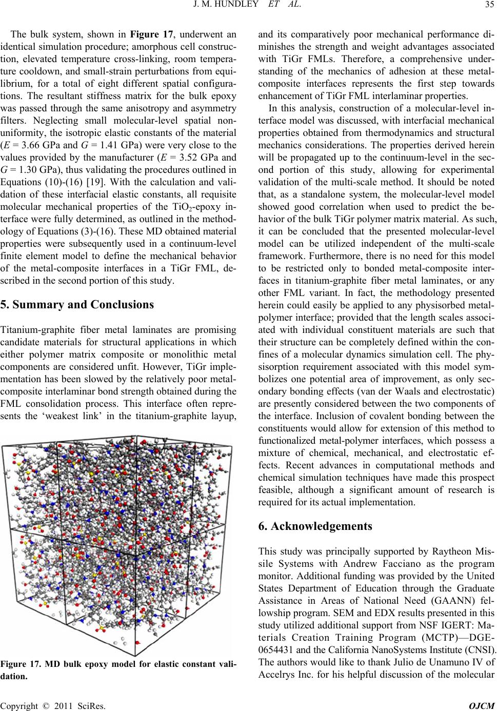 J. M. HUNDLEY ET AL. 35 The bulk system, shown in Figure 17, underwent an identical simulation procedure; amorphous cell construc- tion, elevated temperature cross-linking, room tempera- ture cooldown, and small-strain perturbations from equi- librium, for a total of eight different spatial configura- tions. The resultant stiffness matrix for the bulk epoxy was passed through the same anisotropy and asymmetry filters. Neglecting small molecular-level spatial non- uniformity, the isotropic elastic constants of the material (E = 3.66 GPa an d G = 1.41 GPa) were very close to the values provided by the manufacturer (E = 3.52 GPa and G = 1.30 GPa), thus va lidating th e procedu res outlined in Equations (10)-(16) [19]. With the calculation and vali- dation of these interfacial elastic constants, all requisite molecular mechanical properties of the TiO2-epoxy in- terface were fully determined, as outlined in the method- ology of Equations (3)-(16). These MD obtained material properties were subsequently used in a continuum-level finite element model to define the mechanical behavior of the metal-composite interfaces in a TiGr FML, de- scribed in the second portion of th is study. 5. Summary and Conclusions Titanium-graphite fiber metal laminates are promising candidate materials for structural applications in which either polymer matrix composite or monolithic metal components are considered unfit. However, TiGr imple- mentation has been slowed by the relatively poor metal- composite interlaminar bond strength obtained during the FML consolidation process. This interface often repre- sents the ‘weakest link’ in the titanium-graphite layup, Figure 17. MD bulk epoxy model for elastic constant vali- dation. and its comparatively poor mechanical performance di- minishes the strength and weight advantages associated with TiGr FMLs. Therefore, a comprehensive under- standing of the mechanics of adhesion at these metal- composite interfaces represents the first step towards enhancement of TiGr FML int erlaminar properties. In this analysis, construction of a molecular-level in- terface model was discussed, with interfacial mechanical properties obtained from thermodynamics and structural mechanics considerations. The properties derived herein will be propagated up to the continuum-level in the sec- ond portion of this study, allowing for experimental validation of the multi-scale method. It should be noted that, as a standalone system, the molecular-level model showed good correlation when used to predict the be- havior of the bulk TiGr polymer matrix material. As such, it can be concluded that the presented molecular-level model can be utilized independent of the multi-scale framework. Furthermore, there is no need for this model to be restricted only to bonded metal-composite inter- faces in titanium-graphite fiber metal laminates, or any other FML variant. In fact, the methodology presented herein could easily be applied to any physisorbed metal- polymer interface; provided that the length scales associ- ated with individual constituent materials are such that their structure can be completely defined within the con- fines of a molecular dynamics simulation cell. The phy- sisorption requirement associated with this model sym- bolizes one potential area of improvement, as only sec- ondary bonding effects (van der Waals and electrostatic) are presently considered between the two components of the interface. Inclusion of covalent bonding between the constituents would allow for extension of this method to functionalized metal-polymer interfaces, which possess a mixture of chemical, mechanical, and electrostatic ef- fects. Recent advances in computational methods and chemical simulation techniques have made this prospect feasible, although a significant amount of research is required for its actual implementation. 6. Acknowledgements This study was principally supported by Raytheon Mis- sile Systems with Andrew Facciano as the program monitor. Additional funding was provided by the United States Department of Education through the Graduate Assistance in Areas of National Need (GAANN) fel- lowship program. SEM and EDX results presented in this study utilized additional support from NSF IGERT: Ma- terials Creation Training Program (MCTP)—DGE- 0654431 and the California NanoSystems Institute (CNSI). The authors would like to thank Julio de Unamuno IV of Accelrys Inc. for his helpful discussion of the molecular Co pyright © 2011 SciRes. OJCM  J. M. HUNDLEY ET AL. 36 dynamics simulations employed in this study. Addition- ally, special thanks go to Rachel Hundley for her in- valuable editorial comments. 7. References [1] J. W. Gunnink, A. Vlot, T. J. de Vries and W. van der Hoeven, “Glare Technology Development 1997-2000,” Applied Composite Materials, Vol. 9, No. 4, 2002, pp. 201-219. doi:10.1023/A:1016006314630 [2] J. L. Miller, D. J. Progar, W. S. Johnson and T. L. St. Clair, “Preliminary Evaluation of Hybrid Titanium Com- posite Laminates,” NASA TM-109095, 1994. [3] C. A. J. R. Vermeeren, T. Beumler, J. L. C. G. de Kanter, O. C. van der Jagt and B. C. Out, “Glare Design Aspects and Philosophies,” Applied Composite Materials, Vol. 10, No. 4, 2003, pp. 257-276. doi:10.1023/A:1025581600897 [4] S. Bernhardt, M. Ramulu and A. S. Kobayashi, “Low- Velocity Impact Response Characterization of a Hybrid Titanium Composite Laminate,” Journal of Engineering Materials and Technology, Vol. 129, No. 4, 2007, pp. 220-226. doi:10.1115/1.2400272 [5] H. S. Seo, J. M. Hundley, H. T. Hahn and J. M. Yang, “Numerical Simulation of Glass-Fiber-Reinforced Alu- minum Laminates with Diverse Impact Damage,” Ameri- can Institute of Aeronautic s and A stronautics Jo urnal, Vol . 48, No. 3, 2010, pp. 676-687. doi:10.2514/1.45551 [6] L. B. Greszczuk, “Stress Concentrations and Failure Cri- teria for Orthotropic and Anisotropic Plates with Circular Openings,” Proceedings of the Composite Materials Test- ing and Design 2nd Conference, Anaheim, 1971, pp. 363- 381. [7] J. M. Hundley, H. T. Hahn, J. M. Yang and A. B. Fac- ciano, “Three-Dimensional Progressive Failure Analysis of Bolted Titani um-Graphite Fiber Metal Laminate Joints,” Journal of Composite Materials, Vol. 45, No. 7, 2011, pp. 751-769. doi:10.1177/0021998310391047 [8] B. Kolesnikov, L. Herbeck, and A. Fink, “CFRP/Tita- nium Hybrid Material for Improving Composite Bolted Joints,” Composite Structures, Vol. 83, 2007, pp. 368-380. doi:10.1016/j.compstruct.2007.05.010 [9] R. G. J. van Rooijen, J. Sinke, T. J. de Vries and S. van der Zwaag, “The Bearing Strength of Fiber Metal Lami- nates,” Journal of Composite Materials, Vol. 40, No. 1, 2008, pp. 5-19. doi:10.1177/0021998305053509 [10] G. Lawcock, L. Ye, Y. W. Mai and C. T. Sun, “The Ef- fect of Adhesive Bonding Between Aluminum and Com- posite Prepreg on the Mechanical Properties of Carbon- Fiber-Reinforced Metal Laminates,” Composites Science and Technology, Vol. 57, 1997, pp. 5-45. doi:10.1016/S0266-3538(96)00107-8 [11] G. Wu, J. M. Yang and H. T. Hahn, “The Impact Proper- ti es and Damage Tolerance of Bi-Directionally Reinforced Fiber Metal Laminates,” Journal of Materials Science, Vol. 42, No. 3, 2007, pp. 948-957. doi:10.1007/s10853-006-0014-y [12] T. Q. Cobb, W. S. Johnson, S. E. Lowther and T. L. St. Clair, “Optimization of Surface Treatment and Adhesive Selection for Bo nd Durability in Ti-15-3 La minates,” Jour- nal of Adhesion, Vol. 71, 1999, pp. 115-141. doi:10.1080/00218469908014844 [13] P. Molitor, V. Barron and T. Young, “Surface Treatment of Titanium for Adhesive Bonding to Polymer Compos- ites: A Review,” Journal of Adhesion and Adhesives, Vol. 21, 2001, pp. 129-136. doi:10.1016/S0143-7496(00)00044-0 [14] S. E. Lowther, C. Park and T. L. St. Clair, “A Novel Sur- face Treatment for Titanium Alloys,” NASA TM-99-22, 1999. [15] C. Ohara, T. Hongo, A. Yamazaki and T. Nagoya, “Syn- thesis and Characterization of Brookite/Anatase Complex Thin Film,” Applied Surface Science, Vol. 254, 2008, pp. 6619-6622. doi:10.1016/j.apsusc.2008.04.030 [16] Joint Committee on Powder Diffraction Standards— International Center for Diffraction Data, “Powder Dif- fraction File Card Number 44-1294,” Powder Diffraction File, 1996. [17] Joint Committee on Powder Diffraction Standards— International Center for Diffraction Data, “Powder Dif- fraction File Card Number 21-1276,” Powder Diffraction File, 1996. [18] J. M. Hundley, J. M. Yang, H. T. Hahn and A. B. Fac- ciano, “Bearing Strength Analysis of Hybrid Titanium Composite Laminates,” American Institute of Aeronautics and Astronautics Journal, Vol. 46, No. 8, 2008, pp. 2074- 2085. doi:10.2514/1.36242 [19] Cytec Engineered Materials, “CYCOM 977-3 Toughened Epoxy Resin Technical Datasheet,” 2005. [20] Accelrys Inc., “Materials Studio User’s Manual,” Version 4.4, 2008. [21] H. Sun, “COMPASS: An ab Initio Force-Field Optimized for Condensed-Phase Applications, Overview with De- tails on Alkane and Benzene Compounds,” Journal of Physical Chemistry B, Vol. 102, No. 38, 1998, pp. 7338- 7364. doi:10.1021/jp980939v [22] D. W. Kim, N. Enomoto, Z. E. Nakagawa and K. Kawa- mure, “Molecular Dynamic Simulation in Titanium Di- oxide Polymorphs: Rutile, Brookite and Anatase,” Jour- nal of the American Ceramic Society, Vol. 79, No. 4, 1996, pp. 1095-1099. doi:10.1111/j.1151-2916.1996.tb08553.x [23] H. Knözinger, “Specific Poisoning and Characterization of Catalytically Active Oxide Surfaces,” Advances in Catalysis, Vol. 25, 1976, 184-271. doi:10.1016/S0360-0564(08)60315-6 [24] W. Zhao, “Modeling of Ultrasonic Processing,” MS the- sis, Massachusetts Institute of Technology, Cambridge, 2005. [25] I. Yarovsky and E. Evans, “Computer Simulation of Structure and Properties of Crosslinked Polymers: Ap- plication to Epoxy Resins,” Polymer, Vol. 43, 2002, pp. 963-969. doi:10.1016/S0032-3861(01)00634-6 Copyright © 2011 SciRes. OJCM  J. M. HUNDLEY ET AL. Copyright © 2011 SciRes. OJCM 37 [26] S. Kisin, J. B. Vukić, P. G. T. van der Varst, G. de With and G. C. E. Koning, “Estimating the Polymer-Metal Work of Adhesion from Molecular Dynamics Simulations,” Chemistry of Materials, Vol. 19, 2007, pp. 903- 907. doi:10.1021/cm0621702 [27] I. Yarovsky, “Atomistic Simulation of Interfaces in Ma- terials: Theory and Applications,” Australian Journal of Physics, Vol. 50, 1997, pp. 407-424. [28] D. J. Henry, C. A. Lukey, E. Evans and I. Yarovsky, “Theoretical Study of Adhesion between Graphite, Poly- ester and Silica Surfaces,” Molecular Simulation, Vol. 39, No. 6-7, 2005, pp. 449-455. doi:10.1080/089270412331332712 [29] D. N. Theodorou and U. W. Suter, “Atomistic Modeling of Mechanical Properties of Polymeric Glasses,” Mac- romolecules, Vol. 19, 1986, pp. 139-154.
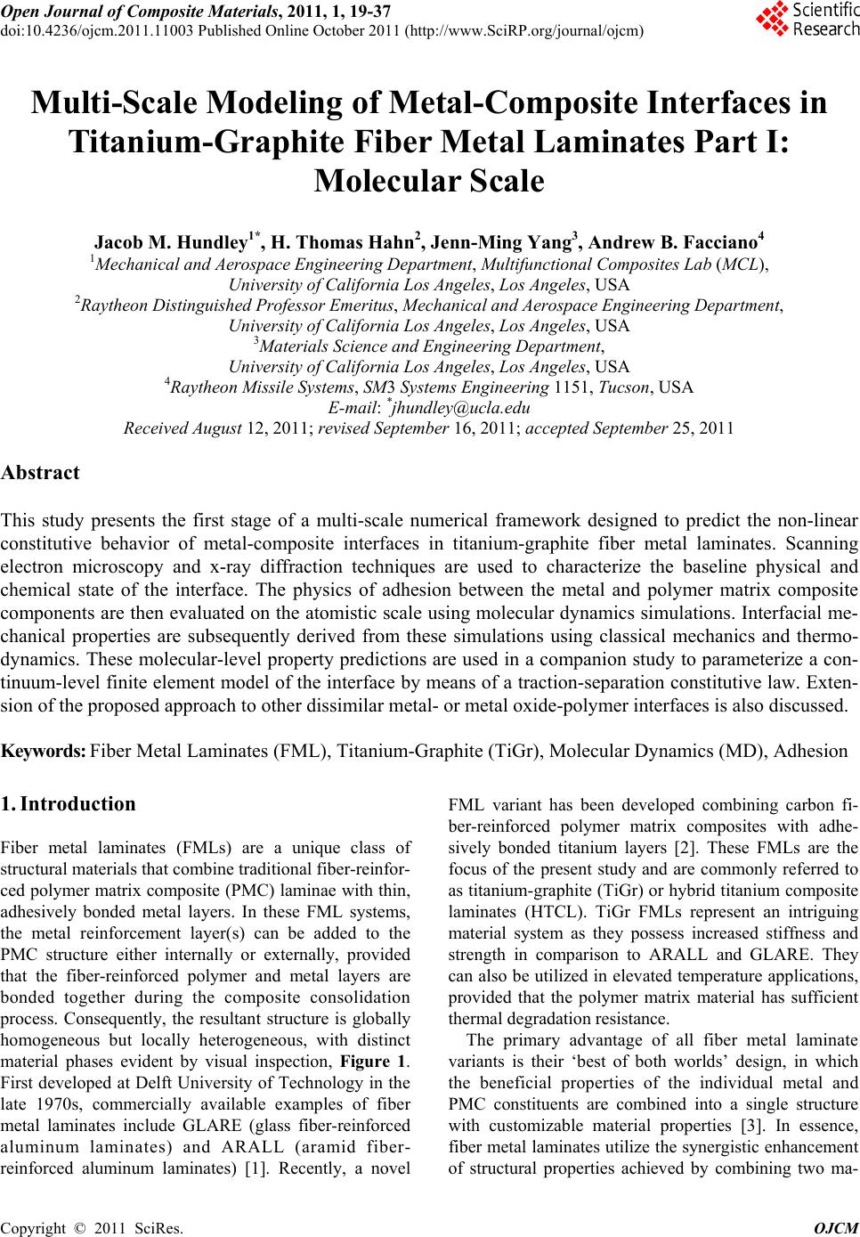
|