Journal of Information Security, 2011, 2, 158-168
doi:10.4236/jis.2011.24016 Published Online October 2011 (http://www.SciRP.org/journal/jis)
Anomalous Network Packet Detection Using
Data Stream Mining
Zachary Miller, William Deitrick, Wei Hu*
Department of Computer Science, Houghton College, Houghton, USA
Received July 4, 2011; revised July 29, 2011; accepted August 8, 2011
Abstract
In recent years, significant research has been devoted to the development of Intrusion Detection Systems
(IDS) able to detect anomalous computer network traffic indicative of malicious activity. While signature-
based IDS have proven effective in discovering known attacks, anomaly-based IDS hold the even greater
promise of being able to automatically detect previously undocumented threats. Traditional IDS are gener-
ally trained in batch mode, and therefore cannot adapt to evolving network data streams in real time. To re-
solve this limitation, data stream mining techniques can be utilized to create a new type of IDS able to dy-
namically model a stream of network traffic. In this paper, we present two methods for anomalous network
packet detection based on the data stream mining paradigm. The first of these is an adapted version of the
DenStream algorithm for stream clustering specifically tailored to evaluate network traffic. In this algorithm,
individual packets are treated as points and are flagged as normal or abnormal based on their belonging to
either normal or outlier clusters. The second algorithm utilizes a histogram to create a model of the evolving
network traffic to which incoming traffic can be compared using Pearson correlation. Both of these algo-
rithms were tested using the first week of data from the DARPA’99 dataset with Generic HTTP, Shell-code
and Polymorphic attacks inserted. We were able to achieve reasonably high detection rates with moderately
low false positive percentages for different types of attacks, though detection rates varied between the two
algorithms. Overall, the histogram-based detection algorithm achieved slightly superior results, but required
more parameters than the clustering-based algorithm. As a result of its fewer parameter requirements, the
clustering approach can be more easily generalized to different types of network traffic streams.
Keywords: Anomaly Detection, Clustering, Data Stream Mining, Intrusion Detection System, Histogram,
Payload
1. Introduction
Since the 1990’s, internet usage has become an integral
part of our daily lives. As a result, computer networks
have experienced an increased number of sophisticated
malware attacks. Whereas attackers previously attempted
to gain access to restricted resources to demonstrate their
skill, a new wave of internet-based attacks has shifted the
focus primarily towards criminal motives. Due to the
availability of software tools designed to exploit vulner-
abilities, attackers can create viruses with greater struc-
tural complexity and damaging capability using less so-
phisticated skills. The security challenges resulting from
an increasing number of devices connected to the inter-
net has prompted a significant amount of research de-
voted to network security.
1.1. Intrusion Detection Systems
One notable topic of network security research is the
development of Intrusion Detection Systems (IDS),
which attempt to detect threats to a network or host
through signature-based or anomaly-based methods. To
detect intrusions, signature-based IDS generate “signa-
tures” based on characteristics of previous known attacks.
This allows the systems to focus on detecting attacks
regardless of ordinary network traffic. Signature-based
detection is the most common form of intrusion detection
because it is simple to implement once a set of signatures
has been created. Although this approach is effective in

159 Z. MILLER ET AL.
finding known threats to a network, it is unable to iden-
tify new threats until a new signature is made. To gener-
ate an accurate signature, a human expert is generally
needed because this cannot easily be done automatically.
Since the detection of new threats in a signature-based
system is impossible without the aid of a new signature,
an alternative method has been proposed.
In contrast to the signature-based approach, anomaly-
based IDS adaptively detect new attacks by first gener-
ating a “normal” pattern of network traffic. These sys-
tems then find anomalies by comparing incoming pack-
ets with the “normal” model. Anything that is considered
statistically deviant is classified as anomalous. This al-
lows for the systems to automatically detect new attacks
though risking possible misclassification of normal be-
havior(false positive).In addition to the potential for false
positives, anomaly-based systems also fall prey to
“mimicry attacks”, which attempt to evade the IDS by
imitating normal network traffic. One such attack is
known as a Polymorphic Blending Attack (PBA), in
which the attacker uses byte padding and substitution to
avoid detection [1]. Recent research has focused on in-
creasing the efficiency, robustness, and detection rates of
these systems while lowering their often high false-posi-
tive rates.
One of the first well-developed anomaly-based sys-
tems is NIDES [2], which builds a model of normal be-
havior by monitoring the four-tuple header of packets.
The four-tuple contains the source and destination IP
addresses and port numbers of packet headers [3]. An-
other system proposed by Mahoney et al. [4] was com-
prised of two different programs, PHAD and ALAD.
Whereas PHAD monitors the data contained in the
header fields of individual packets, ALAD looks at dis-
tinct TCP connections consisting of multiple packets [3,
4]. To detect anomalies, PHAD and ALAD use port
numbers, TCP flags, and keywords found in the payload.
Yet another approach, known as NETAD [5], monitors
the first 48 bytes of each IP packet header and creates
different models based on each individual network pro-
tocol. Then, using the information recovered from the
packet’s header, NETAD creates different models each
corresponding to a particular network protocol [6].
Two recently developed network anomaly-based in-
trusion detection systems are PAYL and McPAD [6,7].
Both used n-grams, sequences of n consecutive bytes in a
packet’s payload, as features to represent packets
To perform anomaly detection, PAYL utilizes 1-grams.
This system first generates a histogram for normal traffic,
and then a new histogram for each packet’s payload. The
two histograms are compared using the simplified Ma-
halanobis distance. If the distance is above a certain
threshold, the new packet is flagged as anomalous [7].
Despite this approach’s effectiveness, it suffers from a
high false positive rate. To combat this, an extension of
PAYL was proposed to use n-grams, creating a more
precise detection model [8].
McPAD further develops the effectiveness of the n-
gram version of PAYL by using 2-nu-grams, sequences
of two bytes separated by a gap of size nu. The 2-gram
contains the correlation between two bytes, a feature that
1-gram lacks. By combining the 2-gram with nu, McPAD
is able to analyze structural information from higher n-
grams while keeping the number of features the same as
a 2-gram.By varying the value of nu, McPAD builds
multiple one-class support vector machine (SVM) classi-
fiers to detect anomalies as an ensemble. These classifi-
ers are first trained on anomaly free data then tested with
mixed normal and abnormal packets [6]. Using this ap-
proach, McPAD has successfully detected multiple virus
types while maintaining a low false positive rate.
1.2. Stream Data Mining
Although PAYL and McPAD have been able to achieve
desirable results, they are not designed to deal with the
gradual or abrupt change in the data flows. Also because
of the Internet’s high speed, systems such as PAYL and
McPAD can not efficiently store and evaluate the large
amount of traffic generated in real-time. To counter these
issues, we propose the application of data stream mining
techniques to anomaly detection.
Stream mining differs from the traditional batch set-
ting in a number of ways. First and foremost, because
data streams are of extremely large or even infinite size,
individual objects within the stream may only beana-
lyzed once—not repeatedly as is possible in batch mode
[9]. The continuous nature of data streams also places
significant time constraints on stream mining solutions.
For a stream mining approach to be practical and effec-
tive, it must be able to process incoming information as
quickly as it arrives [10].
One of the salient features of any data stream mining
algorithm is the ability to detect fluctuations within a
continuous stream of data over an unknown length of
time. This dynamic tendency of streaming data is called
“concept drift” when a change occurs gradually, or “con-
cept shift” when it occurs more quickly [10]. To deal with
this characteristic of streaming data, many stream mining
algorithms employ a window of time intervals to tempo-
rarily hold the most recent data points in a stream [10,11].
The three types of windows typically implemented are
landmark window, sliding window and damped window
[11].

Z. MILLER ET AL.
160
2. Materials and Methods
2.1. Data
Two publicly available datasets were used to evaluate the
anomaly detection algorithms proposed in this study.
These were the DARPA’99 intrusion detection evalua-
tion dataset (http://www.ll.mit.edu/mission/communica-
tions/ist/corpora/ideval/data/1999data.html), and the at-
tack dataset provided by [6].
The DARPA’99 dataset was used to provide a sam-
pling of normal network traffic. This dataset simulates
network communication from a fictitious United States
Air Force base [12], and provides both attack-free and
attack-containing network traces. Data samples for this
study were obtained from HTTP requests found in out-
side tcp dump data for each day from week one of the
DARPA’99 dataset. This first week of data is provided
for training purposes and contains no anomalous network
traffic. Using Jpcap, a free Java-based library for net-
work packet manipulation, (http://netresearch.ics.uci.edu/
kfujii/Jpcap/doc/), the numeric character values for all
HTTP packet payloads with lengths at least 1400 char-
acters were extracted for each day. The resulting dataset
provided a total of 5594 packets representing normal
network traffic divided by days as is shown in Table 1.
The anomalous data used in this study were compiled
by [6], and are freely available online (http://roberto.
perdisci.com/projects/mcpad). We chose to analyze the
algorithms’ performance in the detection of three out of
the four attack types provided: Generic HTTP Attacks,
Shell-code Attacks, and CLET Shell-code attacks. [6]
obtained 63 of the attacks included in their Generic
HTTP dataset from [13]. These attacks include a variety
of HTTP attacks collected in a live environment from
test web servers, as well as various archives and data-
bases. The attacks fall into several categories, including
buffer overflow, URL decoding error, and input valida-
tion error, and were directed against numerous web serv-
ers such as Microsoft IIS, Apache, Active Perl ISAPI,
CERN 3.0A, etc. [6] further supplements these attacks,
bolstering the dataset to include a total of 66 HTTP
threats. The Shell-code attack dataset includes 11 shell-
Table 1. Packets Extracted from DARPA’99 Week 1.
Day Number of Packets
Monday 688
Tuesday 968
Wednesday 860
Thursday 2308
Friday 770
Total 5,594
code attacks (attacks with packets containing executable
code in their payload), which are also included in the
Generic HTTP attack dataset. Finally, the CLET attacks
were generated by [6] using the CLET polymorphic shell-
code engine [14]. This created 96 polymorphic shell-code
attacks containing ciphered data meant to evade pattern-
matching based detection techniques.
Following the same procedure used to process the
DARPA’99 week one data, the numeric character values
contained in all HTTP packet payloads from each of the
three attack datasets with lengths of at least 1400 char-
acters were extracted using Jpcap. This provided a total
of 843 attack packets, with varying numbers of packets
from each attack type as is detailed in Table 2.
The payload information extracted from the DARPA
and attack datasets was used to create training and testing
datasets for our anomaly detection systems. For each of
the five days in the DARPA dataset, 20% of the day’s
packets were extracted to be used for training, and the
remaining 80% of the day’s data were set aside to be
used for testing. To simulate the network traffic in real
time, anomalous packets were then sporadically inserted
into both the training and testing data after an initial in-
terval consisting of only normal traffic (50 packets for
training data and 200 packets for testing data).In this way,
different datasets were created with each attack type for
all five days of DARPA’99 week one (See Figure 1).
The total number of abnormal packets inserted into both
the training and testing data was no more than 10% of all
normal data for the given day with payload length 1400
characters or more. In some cases, as shown in Table 3
and Table 4, the number of abnormal packets inserted
into data was less than 10% because there was not
enough attack data available for that day. For the training
data, 20% of the abnormal data was mixed with 20% of
the normal data for each day. Likewise, 80% of the ab-
normal data was mixed with 80% of the normal data se-
lected from each day for testing. For each packet, 256 1-
gram and 65,536 2-gram features were extracted to pro-
duce separate representations of the training and testing
datasets detailed in Table 3 and Table 4. The datasets
were stored in the ARFF file format used the by the open
source machine learning software WEKA [15].
The payload information extracted from the DARPA
and attack datasets was used to create training and testing
Table 2. Packets extracted from McPAD attack datasets.
Attack TypeNumber of Packets
Generic HTTP122
Shell-code73
CLET Shell-code648
Total843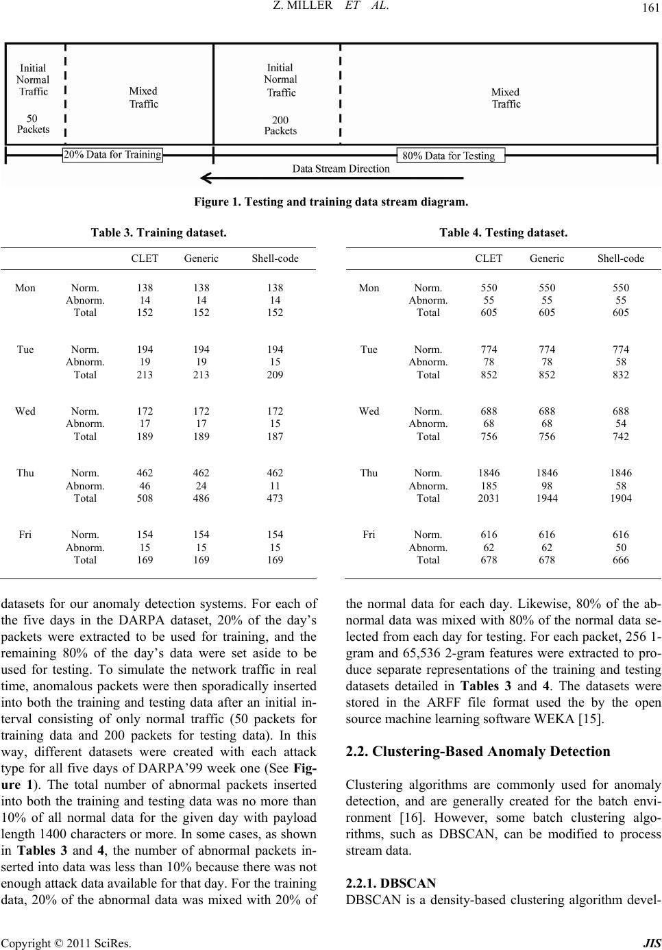

Z. MILLER ET AL.
161
Figure 1. Testing and training data stream diagram.
Table 4. Testing dataset. Table 3. Training dataset.
CLET Generic Shell-code
Mon
Norm.
Abnorm.
Total
138
14
152
138
14
152
138
14
152
Tue Norm.
Abnorm.
Total
194
19
213
194
19
213
194
15
209
Wed
Norm.
Abnorm.
Total
172
17
189
172
17
189
172
15
187
Thu Norm.
Abnorm.
Total
462
46
508
462
24
486
462
11
473
Fri Norm.
Abnorm.
Total
154
15
169
154
15
169
154
15
169
CLET Generic Shell-code
Mon
Norm.
Abnorm.
Total
550
55
605
550
55
605
550
55
605
Tue Norm.
Abnorm.
Total
774
78
852
774
78
852
774
58
832
Wed
Norm.
Abnorm.
Total
688
68
756
688
68
756
688
54
742
Thu Norm.
Abnorm.
Total
1846
185
2031
1846
98
1944
1846
58
1904
Fri Norm.
Abnorm.
Total
616
62
678
616
62
678
616
50
666
datasets for our anomaly detection systems. For each of
the five days in the DARPA dataset, 20% of the day’s
packets were extracted to be used for training, and the
remaining 80% of the day’s data were set aside to be
used for testing. To simulate the network traffic in real
time, anomalous packets were then sporadically inserted
into both the training and testing data after an initial in-
terval consisting of only normal traffic (50 packets for
training data and 200 packets for testing data). In this
way, different datasets were created with each attack
type for all five days of DARPA’99 week one (See Fig-
ure 1). The total number of abnormal packets inserted
into both the training and testing data was no more than
10% of all normal data for the given day with payload
length 1400 characters or more. In some cases, as shown
in Tables 3 and 4, the number of abnormal packets in-
serted into data was less than 10% because there was not
enough attack data available for that day. For the training
data, 20% of the abnormal data was mixed with 20% of
the normal data for each day. Likewise, 80% of the ab-
normal data was mixed with 80% of the normal data se-
lected from each day for testing. For each packet, 256 1-
gram and 65,536 2-gram features were extracted to pro-
duce separate representations of the training and testing
datasets detailed in Tables 3 and 4. The datasets were
stored in the ARFF file format used the by the open
source machine learning software WEKA [15].
2.2. Clustering-Based Anomaly Detection
Clustering algorithms are commonly used for anomaly
detection, and are generally created for the batch envi-
ronment [16]. However, some batch clustering algo-
rithms, such as DBSCAN, can be modified to process
stream data.
2.2.1. DBSCAN
DBSCAN is a density-based clustering algorithm devel-

Z. MILLER ET AL.
162

}
oped for the batch setting. The algorithm takes two user-
defined parameters, epsilon (ε) and minimum points, and
relies on the concepts of ε-neighborhood and core-ob-
jects. An ε-neighborhood is defined by DBSCAN as be-
ing a set of points that have a distance to another point
less than the user-defined parameter ε. More specifically,
given point p and dataset D, the ε-neighborhood of
p is equal to:


Np

 
{,Np qDdistpq


 ∣, (1)
where is the Euclidean distance between
points p and q [17].

,distp q

A core-object is defined as a set of points within an ε-
neighborhood that contain more points than the mini-
mum points parameter. If p is part of a core-object,
DBSCAN will expand the cluster around p.
The basic structure of the algorithm is as follows:
1) DBSCAN takes the ε and minimum points parame-
ters and then chooses a point p that has not been visited.
2) DBSCAN calculates . If the size of

Np

N

is greater than minimum points, DBSCAN expands
a cluster around p. Otherwise, the point is considered
noise.

p
3) DBSCAN iterates to a new un-visited point and re-
peats the process [18].
Although DBSCAN was originally developed for a
batch environment, it has provided an inspiration for
stream clustering algorithms.
2.2.2. De nStream
DenStream is a stream clustering algorithm based on
DBSCAN with a damped window model. It expands the
concept of an ε-neighborhood in DBSCAN with a fading
function to maintain up-to-date information about the
data stream. The fading function is defined as:

2t ft


, (2)
where 0

 represents the decay factor and t repre-
sents the time.
DenStream also modifies the core-object concept of
DBSCAN, creating a core-micro-cluster with three addi-
tional attributes: radius, center and weight. The radius
must be less than or equal to ε, and the weight of a clus-
ter must be greater than the user-defined parameter µ
[11]. The weight w, center c and radius r of a core-micro-
cluster are more formally defined at time t, for a set of
close points, with time-stamps
as:
12
,,,
n
pp p12 ,,,TT
n
T

1
n
i
i
wftT




, (3)

1
n
ii
i
f
tTp
cw

,

1(,)
n
ii
i
f
tTdist pc
rw

, (5)


,
i
distpc
i and the center
where is the Euclidean distance between the
point p c.
Because DenStream operates in a stream environment,
e-micro-cl
e this, a potential core-micro-
cl
the corusters need to change dynamically as
time passes. To facilitat
uster or p-micro-cluster is introduced. P-micro-clusters
are similar to core-micro-clusters, except they differ in
that the center and radius values are based on the
weighted sum and squared sum of the points (1
CF and
2
CF ). Also, the weight must be greater than or equal to

 where

defines the threshold between icro-
clusters and outliers(described in the next praph)
that 01
p-m
arag
such


. 1 CF and 2 CF are calculated us-
ing the formulas:

n
ii
C fp
, (6)
1
1 i
Ft T



22
1
n
ii
i
CFf tTp


. (7)
This changes the center and radius values to be [11,
19]:
1
CF
cw , (8)
2
21
CF



. (9) and CF rww 

Although theicro-cluster permits t
updated dynam, it generally will not
resentative view of a data stream as new points appear.
To
ew point p arrives in the
str
rge p with the closest
p-
an or equal to the value of ε, the point is merged.
Th
p-mhe model to be
ically provide a rep-
handle this concept drift, DenStream also introduces
the outlier-micro-cluster (or o-micro-cluster) and an out-
lier-buffer that temporarily stores o-micro-clusters and
allows them to become p-micro-clusters. The operation
of DenStream is as follows:
Initial Step: run DBSCAN on a set of initial points to
generate starting p-micro-clusters.
Online Steps, when a n
eam:
1) The algorithm attempts to me
micro-cluster. If the radius of the potential micro-cluster
is less th
2) If the point is not merged to a p-micro-cluster, it
tries to merge p with an existing o-micro-cluster. If the
radius is less than ε, it is merged with the o-micro-cluster.
en if the o-micro-cluster now has a weight large
enough to become its own p-micro-cluster, it is removed
(4)

Z. MILLER ET AL. 163
ier-buffer.
is done using the formula:
from the outlier-buffer and added to the model as a p-
micro-cluster.
3) If the point cannot be merged to an existing o-mi-
cro-cluster, it creates a new o-micro-cluster and gets
placed in the outl
After the merging phase of the DenStream algorithm,
the lower weight limit is calculated for all o-micro-clus-
ters in the outlier buffer. This



0
0
21
,
21
cp
p
ttT
cT
tt






, (10)
where 0

 represents the decay factor, t and t rep-
resent the current and starting time for th
ter, and Tp is the predetermined time-period.
the w
ckets, DenStream was modified
create the DenStreamDetection algorithm, which treats
hen a
2.
odel was created in two steps.
he first step used the training data to find a range for
such as ε and
in Section 2.4. A false
po
ese parameters, models were generated with a range of
false pverall
performance.
nother approach to the detection of anomalous network
aintain
tatistical information about network packet payloads.
stogram-based detection algorithm provides a sim-
le method for classification of network traffic. The al-
rithm 2, creates a histo-
c0
e o-micro-clus-
4) Ifeight of a particular cluster is less than the
lower weight limit, the o-micro-cluster can be removed
from the outlier buffer.
2.2.3. Ou r DenStream- B a sed Detectio n System
To detect anomalous pa
to
incoming packets as points to be clustered. W
packet is merged with a p-micro-cluster, it is classified as
normal. Otherwise, it is sent to the outlier-buffer and
classified as anomalous. The ability for o-micro-clusters
to be promoted to p-micro-clusters was removed because
the majority of the packets clustered to the outlier-buffer
are abnormal packets. If one of these o-micro-clusters
became a p-micro-cluster, the model would be tainted
and therefore unable to differentiate between abnormal
and normal packets.
The basic structure of DenStreamDetectionis shown in
Algorithm 1.
2.4. Creatio n of the Detection Model
The anomaly detection m
T
the parameters in DenStreamDetection
minimum points. Using 50 initial points, multiple Den-
StreamDetection models for each day were created to
find a range of optimal parameters that could be used in
the testing step. We found that ε had a larger impact on
the predictions than the minimum points. During the first
step, different parameter ranges were identified based on
day and abnormal packet type.
The second step used the testing data to make a pre-
diction model, which was evaluated with the sensitivity
and false positive rates defined
sitive is a normal packet classified as abnormal. The
parameters used in this step were 200 initial packets, 10
minimum points and a range of ε values specific to each
day and attack type determined from the first step. Using
Algorithm 1. DenStream Detection algorithm.
th
ositive and sensitivity rates to demonstrate o
2.3. Histogram-Based Anomaly Detection
A
packets has involved the use of histograms to m
s
PAYL is an example of such a system [7], in which a
model is created for known normal packet payloads and
then compared with incoming packet payloads to deter-
mine whether or not the newly arriving packets are
anomalous. Due to the evolutionary nature of streaming
data, it is important that any abnormal packet detection
method is able to update its normal model as concept
drift occurs in the incoming data stream. With this in
mind, we present a histogram-based classification method
capable of modeling dynamic network traffic in real
time.
2.3.1. Algorithm Description
The hi
p
gorithm, summarized in Algo
gramen compassing a “normal” model of the network
packets expected to be encountered. This histogram is
generated by counting the frequency of n-gram features
Algorithm: DenStreamDetection (iniP, minP, ε)
Parameters: iniP: number of initial packets
minP: number of minimum packets in initial p-micro-
clusters
ε: distance threshold
Input: File containing normal and abnormal packets in n-gram
form
Output: Predictions of normal and abnormal packets.
cl
. Try to merge p into its nearest p-micro-cluster c
at.
1. Initialize DenStream using iniP and minP to build p-micro-
usters.
2. As each packet p comes in:
3p
4. if


p
radius c


then
5. Merge p into cp;
6. Classify as normal packet;
7. else
8. Try to merge p into nearest o-micro-cluster c0;
9. if


radius c0


then
Create a new ocluster and insert into outlier-
f
10. Merge p into
c0;
11. Classify as abnormal packet;
12. el e s
13. -micro-
buffer;
14. Classify as abnormal packet;
15. end i
16.end if

Z. MILLER ET AL.
164
ed detection algorithm.
und within packet payloads. To begin classification of
a st
normal packets to construct the normal model histogram.
rom the new
pa
rived since
th
ram-based algorithm requires several
arameters, it is important to note that these are not
wo parameters in particular
am model. If this value is too
sm
tances classi-
fie
Algorithm 2. Histogram-bas
fo
ream of packets, the algorithm first requires x initial
This histogram contains frequency counts from all initial
packets for each possible n-gram attribute. Since we are
attempting to model normal traffic, it is imperative that
no abnormal packets are included when this model is
created or else the model will be contaminated and de-
tection rates will decrease. To effectively reflect the evo-
lutionary nature of network traffic, the same fading func-
tion with decay factor λ used in DenStream is applied to
the histogram after each new packet is processed. This
helps to reduce the impact of outdated stream data. After
the initial histogram has been built, the algorithm can
begin to classify the subsequent packets.
In order to classify an incoming network packet, the
algorithm builds a histogram from the newly arrived
packet’s payload. The histogram generated f
cket is then compared with the normal model histo-
gram (to which the fading function has been applied as
each new packet comes in) by computing the Pearson
correlation value between the two histograms. If the
computed Pearson correlation value is above auser-de-
fined threshold t, the packet is classified as normal; oth-
erwise, the packet is classified as abnormal.
To account for the possibility of concept drift and shift
occurring in data flows, the normal histogram model may
need to be rebuilt using packets that have ar
e initialization of the normal histogram model. This
allows the normal model to stay current, modeling pack-
ets most recently classified as normal. In order to facili-
tate this rebuilding process, the algorithm maintains two
queues of user-defined size containing information from
previously processed normal packets. One of these
queues, of size q, stores the histogram data for the pre-
vious packets, while the other, with size w, stores Pear-
son correlation values computed between the packets and
the normal histogram model. Note that only data for
packets classified as normal are included in these two
queues; any packets classified as abnormal are not taken
into account. If the normal histogram is to be rebuilt, a
set of user-specified conditions must be met, giving the
user control of the rebuilding process. When the model is
rebuilt too often, the algorithm’s efficiency will decrease
significantly; however, if it is not rebuilt enough, accu-
racy will diminish. To determine when rebuilding the
normal model is necessary, the algorithm calculates the
number of Pearson correlation values in the stored queue
that are below the user-defined threshold h. If this count
is found to be of a certain value r, the normal model is
rebuilt using packets stored in the histogram data queue
and the queue containing previous Pearson correlation
values is emptied.
2.3.2. Cr i t i cal Paramete rs
Though the histog
p
equally important. Rather, t
have the greatest effect on the algorithm’s ability to de-
tect anomalous packets.
The first of these most critical parameters is q, the size
of the queue of previously processed instances used to
rebuild the normal histogr
all, the normal histogram model generated when the
model is rebuilt will not take into account a sufficient
number of previously processed packets. This results in
an insufficiently robust model, causing both undesirable
sensitivity values and false positive rates.
While q has a noticeable influence on the effectiveness
of the histogram detection algorithm, t, which defines the
Pearson correlation threshold between ins
d as normal and abnormal, is undoubtedly the most
important parameter. This is understandable, as t directly
controls the classification of each individual instance as
it is processed by the algorithm. Furthermore, t also plays
Algorithm: HistogramDetection (x, w, q, t, r, h, λ)
Parameters: x: number of initial normal packets
w: size of Pearson correlation queue
q: size of rebuild queue
t: classification threshold
r: rebuild count
h: rebuild threshold
λ: decay factor
Input: File crmal packets in n-gram
form
Output: Pred abnormal packets
2. Inqueue b to queue of size w
e w
. As each new packet p arrives
irst(p)
rsonCorrelation(g,c))
h values ≤ h
ar()
as abnormal
ontaining normal and abno
at
dictions of normal an
1. Initialize histogram g using x initial packets
itialize rebuild
3. Initialize Pearson correlation log l to queue of siz
4
5. decay (g)
6. Create histogram c from packet p
7. if pearsonCorrelation(g,c) >t then
8. Classify p as normal
9. b.addF
10. if (b.size() >q) then
11. b.removeLast()
12. end if
13. l.addFirst(pea
14. if (l.size() > w) then
15. l.removeLast()
16. end if
17. Calculate number of packetsn in l wit
18. if n ≥ r then
19. rebuild(g)
20. l.cle
21. else
22. Classify p
23. end if
24. end if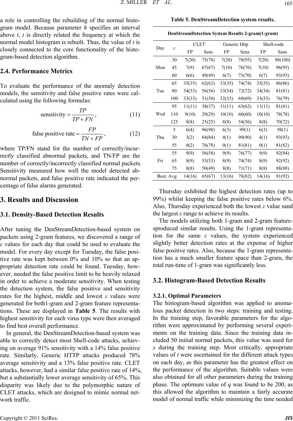

Z. MILLER ET AL. 165
o evaluate the performance of the anomaly detection
se positive rates were cal-
ulated using the following formulas:
a role in controlling the rebuilding of the normal histo-
gram model. Because parameter h specifies an interval
above t, t is directly related the frequency at which the
normal model histogram is rebuilt. Thus, the value of t is
closely connected to the core functionality of the histo-
gram-based detection algorithm.
2.4. Performance Metrics
T
models, the sensitivity and fal
c
sensitivity TP
TP FN
, (11)
false positive rate
F
P
TNFP , (12)

where TP/FN stand for the number of correctly/incur-
rectly classified abnormal packets, and
number of correctly/incorrectly classified normal packets.
.1. Density-Based Detection Results
fter tuning the DenStreamDetection-based system on
ed a range of
ues for each day that could be used to evaluate the
th a 14% false positive
rat
mDetection System Results 2-gram(1-gram)
TN/FP are the
Sensitivity measured how well the model detected ab-
normal packets, and false positive rate indicated the per-
centage of false alarms generated.
3. Results and Discussion
3
A
packets using 2-gram features, we discover
ε val
model. For every day except for Tuesday, the false posi-
tive rate was kept between 0% and 10% so that an ap-
propriate detection rate could be found. Tuesday, how-
ever, needed the false positive limit to be heavily relaxed
in order to achieve a moderate sensitivity. When testing
the detection system, the false positive and sensitivity
rates for the highest, middle and lowest ε values were
generated for both1-gram and 2-gram feature representa-
tions. These are displayed in Table 5. The results with
highest sensitivity for each virus type were then averaged
to find best overall performance.
In general, the DenStreamDetection-based system was
able to correctly detect most Shell-code attacks, achiev-
ing on average 91% sensitivity wi
e. Similarly, Generic HTTP attacks produced 78%
average sensitivity and a 13% false positive rate. CLET
attacks, however, had a similar false positive rate of 14%,
but a substantially lower average sensitivity of 65%. This
disparity was likely due to the polymorphic nature of
CLET attacks, which are designed to mimic normal net-
work traffic.
Table 5. DenStreamDetection system results.
DenStrea
CLET Generic Http Shell-code
Day ε
100)
FP Sens FP Sens FP Sens
307(20)75(78) 7(20) 78(95) 7(20)98(
45 7(967) 7()
60 4
) 67(7(10) )76(7610) 96(95 Mon
6(6) 9(49)6(7) 73(70) 6(7) 93(93)
6535(35) 62(62) 33(35) 74(74) 35(35)86(86)
80 3
33 3
4(33)56(56) 33(34) 72(72) 34(34)81(81)
Tue
1003(33) 51(50)2(33) 69(69) 3(33)76(79)
9511(11) 38(37) 11(11) 63(62) 11(11)81(81)
1109(10) 29(29))10(10 60(60) 10(10)78(78) Wed
125 )8(8 25(25)8(8) 54(56) 8(8) 70(72)
5 6(4) 96(98)6(3) 99(1) 6(3) 98(1)
303(2) 84(84)4(1) 90(90) 4(1) 93(93) Thu
550(2) 76(78)0(1) 81(81) 0(1) 81(82)
559(9) 56(58)9(9) 76(77) 9(9) 92(94)
658(9) 53(53)8(9) 74(74) 8(9) 92(92)
Fri
758(8) 50(49)8(8) 71(71) 8(8) 88(88)
Best. A11 1vg4(16) 65(67)3(16) 78(82) 4(16)91(92)
Thur htioes
9snfalo.
lso, Thursday experienced both the lowest ε value sand
th
em experienced
sli
.2.1. Optimal Parameters
o anoma-
packet detection in two steps: training and testing.
le parameters for the algo-
sday exhibited theighes detectn rat (up to
9%) whil t keepig the alse positive rtes bew 6%
A
e largest ε range to achieve its results.
The models utilizing both 1-gram and 2-gram feature-
sproduced similar results. Using the 1-gram representa-
tion for the same ε values, the syst
ghtly better detection rates at the expense of higher
false positive rates. Also, because the 1-gram representa-
tion has a much smaller feature space than 2-gram, the
total run-time of 1-gram was significantly less.
3.2. Histogram-Based Detection Results
3
The histogram-based algorithm was applied t
lous
In the training step, favorab
rithm were approximated by performing several experi-
ments on the training data. Since the training data in-
cluded 50 initial normal packets, this value was used for
x during the training step. Most critically, appropriate
values of t were ascertained for the different attack types
on each day, as this parameter has the greatest effect on
the performance of the algorithm. Suitable values were
also obtained for all other parameters during the training
phase. The optimum value of q was found to be 200, as
this allowed the algorithm to maintain a fairly accurate
model of normal traffic while minimizing the time needed

Z. MILLER ET AL.
166
tained 200 initial normal
pa
ble to attain
irly consistent results across all days’ testing data for
imal parameters. The algorithm
Histogram Detection System Results 2-gram
attackedod r ra-based
algorit r sd
ratainedalse ositao
maly detection systems is
he evolutionary nature of network
this challenge, we calculated the
to for this model to be rebuilt. Also, 30 was generally
used for w, with r valued at 10 and h at 0.2. These pa-
rameters effectively limited the frequency of rebuilding
the normal histogram model while still allowing the al-
gorithm to handle concept drift in the data. A λ value of
0.01 was found to work sufficiently well, as this decay
factor helped to better maintain an up-to-date normal
model for normal traffic.
Once appropriate parameters were identified, the test-
ing phase began. In this step, the value 200 was assigned
to x since the testing data con
ckets. With the rest of the algorithm’s parameters re-
maining static, the algorithm was tested using varying
values of t in order to gauge sensitivity values at differ-
ent false positive rates. This produced the results sum-
marized in Table 6, which displays a sampling of t val-
ues used for different days and attack types with the re-
sulting sensitivities and false positive rates.
3.2.2. Re s ults Achieve d
As can be seen from Table 6, we were a
fa
each attack type using opt
performed best at detecting shell-code attacks, achieving
an average of 97% sensitivity and 1% false positive rate
across all shell-code attack testing datasets. Performance
was slightly less desirable in detection of Generic HTTP
attacks, but was nevertheless acceptable, with an average
detection rate of 84% and 3% false positive rate. CLET
Table 6. Histogram-based detection system results.
CLET Generic HTTP Shell-code
Day FP Sens
0.0025 0 058
t FP Sens t FP Sens t
25 0.00250 76 0.0005
0.0060 7 31 0.0.008
0.0080 8 0.00900.05
00705 76 10 07 Mon
60 9 76 03096
0.00005 1 27 0.00021 27 0.00001131
0.0025 7 37 0.00102 71 0.0010 279
Tue
0.0035 9 40 0.00152 83 0.0015 297
0.0020 1 29 0.00040 38 0.0005 043
0.0040 2 35 0.00100 66 0.0010 078
Wed
0.0045 3 44 0.00301 81 0.0020 196
0.0050 0 69 0.00050 78 0.0005 097
0.1505 3 98 0.00100 88 0.0755 298
Thu
0.4000 3 100 0.08552 100 0.1000 3100
0.0005 0 26 0.00050 39 0.0010 060
0.0020 2 27 0.00100 61 0.0015 182 Fri
0.0065 13 63 0.00151 79 0.0020 196
Be
s prov mst ifficult fothe histogm
hm to detect. In order foreaonable etection
tes to be ob, fpive rates generally hd t
be pushed much higher than necessary for the other two
attack types, to an average of 7% with optimal parame-
ters. Despite this fact, sensitivity remained comparatively
low, at an average of 61%. This difficulty detecting
CLET attacks was likely due to their polymorphic nature,
which also proved troublesome to the DenStream Detec-
tion system.
While results were relatively consistent across each
days’ worth of training data, those achieved using Thurs-
day’s testing data were markedly superior. Using optimal
parameters, the histogram-based detection algorithm was
able to achieve perfect detection on all three types of
attacks, each with a false positive rate of 3% or less.
There are several possible reasons for this exceptional
performance related to the nature of Thursday’s testing
data as discussed in Section 3.3. Overall, the relatively
high t values used indicate greater consistency in Thurs-
day’s network traffic. Due to these elevated t values, the
algorithm was able to more effectively identify abnormal
network packets.
The number of parameters required by the histogram-
based detection algorithm necessitated fairly specific
tuning for our different datasets in order to perform op-
timally. This was demonstrated by the algorithm’s per-
formance on 1-gram features when the same parameters
used for 2-gram were applied. While the clustering-based
algorithm was able to achieve comparable results from
both 1-gram and 2-gram with the same parameters, the
histogram-based algorithm performed poorly on 1-gram
when applied with the same parameters as 2-gram. As a
result, 1-gram results have not been reported for the his-
togram-based algorithm.
3.3. Concept Shift
he performance of our anoT
heavily influenced by t
affic. To demonstrate tr
Pearson correlation between segments of ten packets for
each day. By measuring the correlation between two
consecutive segments, changes in the stream can be
visualized (Figure 2), which offers a possible explana-
tion to the results observed in Tables 5 and 6.
Monday, Wednesday, and Friday exhibit continuous
concept shift, particularly during the training phase, as
the calculated Pearson correlation values oscillate regu-
larly. Therefore, a robust model for normal traffic was
built in each case that responded accurately to the evolv-
ing data stream. As a result, greater sensitivity was a-
chieved on each of these three days.
st Avg. 7 61 3 84 197

Z. MILLER ET AL.
167
Figure 2. Pearson correlation curves for DARPA’99 week 1.
Tuesday demonstrates a ve
starts with slight shift, but remains relatively stable
th
ed through concept shift. During the training
ph
experienced consistent con-
cept drift, which led to superior detection results.
were
pplied to the problem of anomaly detection. First, a
gorithm was used to detect abnormal
ackets. Using 1-gram and 2-gram features, this ap-
ry distinct pattern, as it Therefore, Thursday likely
roughout the stream. In contrast to Monday, Tuesday
experiences only two major shifts, both of which occur
during the training phase. Therefore, Tuesday’s models
may have a less accurate view of the incoming stream,
causing decreased performance. Since Tuesday only ex-
perienced shift during the training phase, it had a less
accurate view of the changing stream environment. This
may have led to the performance issues stated previ-
ously.
The high sensitivity values for Thursday can also be
explain
ase, consistent concept shift occurred, allowing Thurs-
day’s model to effectively capture the changing pattern
of normal network traffic. Following the training step,
the remainder of Thursday’s data was relatively stable.
4. Conclusions
In this paper, two data stream mining techniques
a
stream clustering al
p
proach achieved moderate success with Generic HTTP
and Shell-code attacks but had a higher average false
positive rate. Second, a stream adaptation of the relative
frequency histogram approach found in [7] was created
using Pearson correlation to detect anomalies.
Though the histogram-based approach achieved mod-
erately better results, it required more fine-tuning be-
cause of the number of parameters used. In contrast,

Z. MILLER ET AL.
168
easi
ac
w
thank the Summer Research Institute at
oughton College for providing funding for our re-
rdisci, G. Gu and W. Lee, “Using an Ensembl
One-Class svm Classifiers to Harden Payload-Based
ction Systems,” ICDM’06: Proceedings of
nation Conference on Data Mining, Hong
generalization of the clustering algorithm waser to
hieve since it uses fewer parameters. This was evi-
denced by the ability of the clustering algorithm to per-
form effectively on both 1-gram and 2-gram features
with the same parameters, while the histogram algorithm
required specific parameter tuning for each feature type.
Lastly, to better explain the performance differences
between certain days, we analyzed the Pearson correla-
tion between consecutive segments of 10 packets. By
plotting these values on a graph, concept drift and shift
ere visualized, and clear variations were observed be-
tween days. The location and frequency of concept shift
and drift in the data streams, especially within the train-
ing phase, provided an account for the observed changes
in performance.
5. Acknowledgements
We would like to
H
search.
6. References
[1] R. Pee of
Anomaly Dete
the Sixth Integ
Kong, 18-22 December 2006, pp. 488-498.
doi:10.1109/ICDM.2006.165
[2] D. Anderson, T. Lunt, H. Javits and A. Tamaru, “Nides:
Detecting Unusual Program Behavior Using the Statisti-
cal Component of the Next Generation Intrusion Detec-
tion Expert System,” Technical Report SRI-CSL-95-06,
P. Chan, “Learning Non Stationary
, P. Fogla, G. Giacinto and W. Lee,
Intrusion Detection,” Recent Advances in Intrusion
Computer Science Laboratory, SRI International, Menlo
Park, May 1995.
[3] R. Perdisci, “Statistical Pattern Recognition Techniques
for Intrusion Detection in Computer Networks, Chal-
lenges and Solutions,” University of Cagliari, Italy, 2006.
[4] M. Mahoney and
Models of Normal Network Traffic for Detecting Novel
Attacks,” ACM SIGKDD International Conference on
Knowledge Discovery and Data Mining, Edmonton, July
2002, pp. 376-385.
[5] M. Mahoney, “Network Trafic Anomaly Detection Based
on Packet Bytes,” ACM-SAC, Melbourne, 2003 pp. 346-
350.
[6] R. Perdisci, D. Ariu
“McPAD: A Multiple Classifier System for Accurate
Payload-based Anomaly Detection,” Computer Networks,
Special Issue on Traffic Classification and Its Applica-
tions to Modern Networks, Vol. 5 No. 6, 2009, pp. 864-
881.
[7] K. Wang and S. Stolfo, “Anomalous Payload-Based Net-
work
Detection (RAID), Vol. 3224, 2004, pp. 203-222.
doi:10.1007/978-3-540-30143-1_11
[8] K. Wang, “Network Payload-Based Anomaly D
and Content-Based Alert Correlation
etection
,” Columbia Univer-
sity, Uppsala, 2011.
ine Learning
m with Noise,”
Evalua-
sity, New York, 2006.
[9] J. Tang, “An algorithm for Streaming Clustering,” MSc.
Thesis, Uppsala Univer
[10] A. Bifet, G. Holmes, R. Kirkby and B. Pfahringer, “MOA:
Massive Online Analysis,” Journal of Mach
Research, Vol. 11, 2010, pp. 1601-1604.
[11] F. Cao, M. Ester, W. Qian and A. Zhou, “Density-Based
Clustering over an Evolving Data Strea
SIAM Conference Data Mining, Bethesda, 2006.
[12] R. Lippmann, J. Haines, D. Fried, J. Korba and K. Das,
“The 1999 DARPA Off-Line Intrusion Detection
tion,” Computer Networks, Vol. 34, No. 4, 2000, pp. 579-
595. doi:10.1016/S1389-1286(00)00139-0
[13] K. L. Ingham and H. Inoue, “Comparing Anomaly Detec-
tion Techniques for HTTP,” Recent Advances in Intru-
Engine Using Spectrum
Edition, Mor-
roceedings of
in Large
al Data,”
Clustering Evolving Data
sion Detection (RAID), 2007.
[14] T. Detristan, T. Ulenspiegel, Y. Malcom and M. Under-
duk, “Polymorphic Shellcode
Analysis,” Phrack, Vol. 11, No. 61, 2003.
[15] I.H. Witten and E. Frank, “Data Mining: Practical Ma-
chine Learning Tools and Techniques,” 2nd
gan Kaufmann Publishers, Waltham, 2005.
[16] L. Portnoy, E. Eskin and S. Stolfo, “Intrusion Detection
with Unlabeled Data Using Clustering,” P
ACM CSS Workshop on Data Mining Applied to Security
(DMSA-2001), Philadelphia, 2001, pp. 333-342.
[17] M. Ester, H. Kriegel, J. Sander and X. Xu, “A Den-
sity-Based Algorithm for Discovering Clusters
Spatial Databases with Noise,” International Conference
on Knowledge Discovery in Databases and Data Mining
(KDD-96), Portland, August 1996, pp. 226-231.
[18] K. Mumtaz and K. Duraiswamy, “An Analysis on Den-
sity Based Clustering of Multi Dimensional Spati
Indian Journal of Computer Science and Engineering,
Vol. 1, No. 1, 2010, pp. 8-12.
[19] A. Forestiero, C. Pizzuti and G. Spezzano, “FlockStream:
a Bio-Inspired Algorithm for
Streams,” ICTAI’09 Proceedings of the 2009 21st IEEE
International Conference on Tools with Artificial Intelli-
gence, Washington DC, 2009, pp. 1-8.