Vol.3, No.10, 817-826 (2011) Natural Science
http://dx.doi.org/10.4236/ns.2011.310107
Bianchi type-VIo Universe with wet dark fluid
Raghavendra Chaubey
DST-Centre for Interdisciplinary Mathematical Sciences, Faculty of Science, Banaras Hindu University, Varanasi, India;
Received 4 February 2011; revised 18 March 2011; accepted 27 March 2011.
ABSTRACT
The Bianchi type-VIo universe filled with dark
energy from a wet dark fluid has been consid-
ered. A new equation of state for the dark en-
ergy component of the universe has been used.
It is modeled on the equation of state =p




 which can describe a liquid, for ex-
ample water. The exact solutions to the corre-
sponding field equations are obtained in quad-
rature form. The solution for constant decelera-
tion parameter have been studied in detail for
power-law and exponential forms both. The
case =0

,=1

and =1 3

have been also
analysed.
Keywords: Cosmological Models; Wet Dark Fluid;
Cosmological Parameters
1. INTRODUCTION
The nature of the dark energy component of the uni-
verse [1-3] remains one of the deepest mysteries of
cosmology. There is certainly no lack of candidates:
cosmological constant, quintessence [4-6], k-essence
[7-9], phantom energy [10-12]. Modifications of the
Friedmann equation such as Cardassian expansion
[13,14] as well as what might be derived from brane
cosmology [15-17] have also been used to explain the
acceleration of the universe. A particular case of the lin-
ear equation of state has used in the cosmological con-
text by Xanthopuolos [18], he considered space-times
with two hypersueface orthogonal, spacelike, commut-
ing killing fields.
In this work, we use Wet Dark Fluid (WDF) as a
model for dark energy. This model is in the spirit of the
generalized Chaplygin gas (GCG) [19], where a physi-
cally motivated equation of state is offered with proper-
ties relevant for the dark energy problem. Here the mo-
tivation stems from an empirical equation of state pro-
posed by Tait [20] and Hayword [21] to treat water and
aqueous solution. The equation of state for WDF is very
simple,


=
WDF WDF
p



 (1.1)
and is motivated by the fact that it is a good approxima-
tion for many fluids, including water, in which the in-
ternal attraction of the molecules makes negative pres-
sures possible. One of the virtues of this model is that
the square of the sound speed, 2
s
c, which depends on
p


, can be positive (as opposed to the case of phan-
tom energy, say), while still giving rise to cosmic accel-
eration in the current epoch.
We treat Eq.1.1 as a phemenological equation [22].
Holman et al. [23] have shown that this model can be
made consistent with the most recent SNIa data [24], the
WMAP results [25,26] as well as constraints coming
from measurements of the matter power spectrum [27].
The parameters

and


are taken to be positive and
we restrict ourselves to 01

. Note that if
s
c de-
notes the adiabatic sound speed in WDF, then 2 =
s
c 
(refer Babichev et al. [28]).
To find the WDF energy density, we use the energy
conservation equation


3=0
WDFWDF WDF
Hp  
 (1.2)
From equation of state (1.1) and using 3=
H
VV
 in
above equation, we have

1
=1
WDF
C
V






 (1.3)
where C is a constant of integration. Here V is vol-
ume expansion.
WDF naturally includes two components: a piece that
behaves as a cosmological constant as well as a standard
fluid with an equation of state =p

 . We can show
that if we take >0C, this fluid will not violate the
strong energy condition 0p


:



1
=1
=10
WDF WDFWDF
p
C
V


 





(1.4)
Chaubey and Chaubey et al. ([29,30]) have studied

R. Chaubey / Natural Science 3 (2011) 817-826 818
Bianchi type-I and V universes with wet dark fluid. In
this paper we study the Bianchi type-VIo universe with
matter term with dark energy treated as a Dark Fluid
satisfying the equation of state (1.1). The solution has
been obtained in the quadrature form. The models with
constant deceleration parameter have been studied in
detail.
2. BASIC EQUATION
We take Bianchi type-VIo metric in form
22
222222 222 2
12 3
=.
mx mx
dsdta dxaedyaedz

 (2.1)
where the metric functions 12 3
,,aa a are functions of t
only and m is a constant
The Einstein field equations for the metric (2.1) are
written in the form
4
1
323 2
1
2
23231
=.
aaa amT
aaaaa
  
   (2.2)
4
2
313 1
2
2
13131
=.
aaa am
T
aaaaa
 
   (2.3)
4
3
1212
3
2
12121
=.
aa aa mT
aa aa a
  
  (2.4)
4
0
23 31 12
0
2
122331 1
=.
aa aa aa mT
aaa aa aa
 
   (2.5)
32
32
=0
aa
aa

 (2.6)
Here  is the gravitational constant and overhead
dot denotes differentiation with respect to t.
The energy-momentum tensor of the source is given
by

=.
j
jj
iWDFWDFiWDF i
Tpuup

  (2.7)
where i u is the flow vector satisfying
=1.
ij
ij
guu (2.8)
In a co-moving system of coordinates, from Eq.2.7
we find
0123
0123
=,===.
WDF WDF
TTTTp   (2.9)
Now using Eq.2.9 in Eqs.2.2-2.6 we obtain
4
323 2
2
23231
=.
WDF
aaa amp
aaaaa
  
   (2.10)
4
313 1
2
13131
=.
WDF
aaa am
p
aaaaa
  
   (2.11)
4
1212
2
12121
=.
WDF
aaaamp
aa aaa
  
 
(2.12)
4
23 31 12
2
122331 1
=.
WDF
aa aa aa m
aaaaaa a
 
   (2.13)
32
32
=0
aa
aa

 (2.14)
From Eq.2.14 we get
23
=aa (2.15)
Let V be a function of t defined by
123
=.Vaaa (2.16)
From Eqs.2.15 and 2.16, we get
2
12
=Vaa (2.17)
Now adding Eqs.2.10-2.12 and three times Eq.2.13,
we get

24
122 12
22
12 12 21
23
22 2=
2WDF WDF
aaaaamp
aa aa
aa


 



(2.18)
From Eqs.2.17 and 2.18 we have

4
2
1
23
=.
2WDF WDF
Vm p
Va



(2.19)
The conservational law for the energy-momentum
tensor gives

=.
WDFWDF WDF
Vp
V
 

 (2.20)
Case 1: When 1=aV
Then Eq.2.19 reduces to

4
23
=.
2WDF WDF
Vm p
VV



(2.21)
From Eqs.2.20 and 2.21 we have
24
1
=3 4
WDF
VC VmV   
 (2.22)
with 1 C being an integration constant.
Rewriting Eq.2.2 0 in the form
=
WDF WDF
V
pV






(2.23)
and taking into account that the pressure and the energy
density obeying an equation of state of type =
WDF
p


WDF
f  , we conclude that WDF

and WDF p, hence
the right hand side of the Eq.2.19 is a function of V
only.
 
4
3
=2.
2WDF WDF
VpVmFV


 (2.24)
From the mechanical point of view Eq.2.24 can be
interpreted as equation of motion of a single particle

R. Chaubey / Natural Science 3 (2011) 817-826
819
819
with unit mass under the force

F
V. Then

=2 .VUV   

 (2.25)
Here

can be viewed as energy and

UV as the
potential of the force
F
. Compairing the Eqs.2.22 and
2.25 we find 1 =2C

and

24
3
=4.
2WDF
UVV mV 




(2.26)
Finally, we write the solution to the Eq.2.22 in quad-
rature form
0
24
1
d=.
34
WDF
Vtt
CVmV 


 (2.27)
where the integration constant 0
t can be taken to be
zero, since it only gives a shift in time.
From Eqs.1.3 and 2.27 we obtain

0
1
24
1
d=.
334
1
Vtt
VCV mVC

 






(2.28)
Case 2: When 2=aV
Then Eq.2.19 reduces to

43
2= .
2WDF WDF
Vmp
V



(2.29)
From Eqs.2.20 and 2.29 we have

42
1
=34
WDF
VC mV   
 (2.30)
with 1 C being an integration constant.
From Eq.2.23 and taking into account that the pres-
sure and the energy density obeying an equation of state
of type

=
WDF WDF
pf 
, we conclude that WDF

and
WDF
p, hence the right hand side of the Eq.2.19 is a func-
tion of V only.
 
4
3
=2.
2WDF WDF
VpVmVFV


 (2.31)
From the mechanical point of view Eq.2.31 can be
interpreted as equation of motion of a single particle
with unit mass under the force

F
V. Then

=2 .VUV  

 (2.32)
Here

can be viewed as energy and

UV as the
potential of the force
F
. Compairing the Eqs.2.30 and
2.32 we find 1 =2C

and

42
3
=4.
2WDF
UVm V 




(2.33)
Finally, we write the solution to the Eq.2.30 in quad-
rature form

0
42
1
d=.
34
WDF
Vtt
CmV



 (2.34)
where the integration constant 0
t can be taken to be
zero, since it only gives a shift in time.
From Eqs.1.3 and 2.34 we obtain

0
1
42
1
d=.
343
1
Vtt
mV CVC

 





 



 (2.35)
3. SOME PARTICULAR CASES
Case 1: When 1=aV
Case I. =0

(Dust Universe)
Eq.2.28 reduces to
4
1
d=
34
2
Vt
CmVC





 (3.1)
which gives
2
42
1
4
32
4
=34
2
CmtC
VCm











(3.2)
From Eqs.2.15, 2.17 and 3.2, we get

12
2
42
1
1
4
32
4
=34
2
CmtC
at Cm

















 



(3.3)
 
14
2
42
1
23
4
32
4
== 34
2
CmtC
at atCm

















 



(3.4)
From Eqs.1.3 and 3.2 we have
1
2
42
1
4
32
4
=34
2
WDF
CmtC
CCm


















 



(3.5)
and from Eqs.1.1 and 3.5 we get
=0
WDF
p (3.6)
The physical quantities of observational interest in
cosmology are the expansion scalar

, the mean ani-
sotropy parameter
A
, the shear scalar 2

and the de-
celeration parameter q. They are defined as [31,32]

R. Chaubey / Natural Science 3 (2011) 817-826 820
=3 .
H

(3.7)
2
3
=1
1
=.
3
i
i
H
AH




 (3.8)

3
2222
=1
13
=3=.
22
i
i
H
HAH  
 (3.9)
d1
=1.
d
qtH



 (3.10)
with the use of Eqs.3.7-3.10 we can express the physical
quantities as
2
4
2
42
1
3
22
4
=
32
4
Cmt
CmtC










(3.11)
1
=8 A (3.12)
2
2
4
2
2
42
1
32
14
=12 32
4
Cmt
CmtC











 



(3.13)
1
2
42
1
=232
4
C
q
Cmt





(3.14)
For large cosmic time, the shear dies out.
Case II. =1

(Zeldovich Fluid)
Eq.2.28 reduces to
24
1
d=
33
4
42
Vt
VmV CC 


 


 (3.15)
which gives

84
1
63 2 6438
=sinh
323
CC mm
Vt
 




 




(3.16)
when

8
1
32
>33 2
m
CC


34
2
28
=3
3
tm
Ve











(3.17)
when

8
1
32
=33 2
m
CC



84
1
6463238
=cosh
323
mCC m
Vt
 




 




(3.18)
when

8
1
32
<33 2
m
CC


We consider these subcases separately.
Case II(a)

8
1
32
=33 2
m
CC


Then

12
34
2
1
28
=3
3
tm
at e











(3.19)
 
14
34
2
23
28
== 3
3
tm
at ate











(3.20)
From Eqs.1.3 and 3.17, we have
2
34
2
28
=23
3
t
WDF
m
Ce














(3.21)
and from Eqs.1.1 and 3.21, we get
2
34
2
28
=23
3
t
WDF
m
pCe











 


(3.22)
with the use of Eqs.3.7-3.10 we can express the physical
quantities as
3
2
34
2
3
2
=
4
3
t
t
e
m
e










(3.23)
1
=8 A (3.24)
2
3
2
2
34
2
3
2
=
4
3
t
t
e
m
e
























(3.25)
3
4
2
43
=1
t
m
qe





 (3.26)
The model has no singularity.
Case II(b)

8
1
32
>33 2
m
CC


Then for small t (i.e. near singularity =0t),

R. Chaubey / Natural Science 3 (2011) 817-826
821
821
33
sinh 22 tt








(3.27)
Then Eq.3.16 reduces to

84
1
3216 8
=233
CC mm
Vt





(3.28)
Then
 
12
84
1
1
3216 8
=233
CC mm
at t








(3.29)
 
14
84
1
23
3216 8
== 233
CC mm
at att








(3.30)
From Eqs.1.3 and 3.28, we have

2
84
1
3216 8
=2233
WDF
CC mm
Ct











(3.31)
and from Eqs.1.1 and 3.21, we get

2
84
1
3216 8
=2233
WDF
CC mm
pC t








 


(3.32)
with the use of Eqs.3.7-3.10 we can express the physical
quantities as


8
1
84
1
3216
23
=
3216 8
233
CC m
CC mm
t









(3.33)
1
=8 A (3.34)


2
8
1
2
84
1
3216
23
1
=48 3216 8
233
CC m
CC mm
t
















(3.35)
=2q (3.36)
The model has no singularity.
Case II(c)
 
8
1
<323 32mCC 

Then for small t (i.e. near singularity =0t),
2
33
cosh 1
24
tt



 


(3.37)
Then Eq.3.18 reduces to


82
1
84
1
3
=432
8
646 328
3
Vm CCt
mCCm









(3.38)
Then
 

82
11
12
84
1
3
=43 2
8
646328
3
atmC Ct
mCCm














(3.39)
 

82
23 1
14
84
1
3
==4 32
8
646 328
3
atatmC Ct
mCCm















(3.40)
From Eqs.1.3 and 3.38, we have


82
1
2
84
1
3
=432
28
646 328
3
WDF Cm CCt
mCCm









 







(3.41)
and from Eqs.1.1 and 3.41, we get


82
1
2
84
1
3
=432
28
646 328
3
WDF
pCmCCt
mCCm








 







(3.42)
with the use of Eqs.3.7-3.10 we can express the physical
quantities as
1
=8 A (3.44)

 
8
1
84
1
82
1
3
163 2
2
=
646 328
3
432
83
mCCt
mCCm
mCCt


 







(3.43)

R. Chaubey / Natural Science 3 (2011) 817-826 822

 
2
8
1
2
84
1
82
1
3
163 2
12
=48 646 328
3
432
83
mCCt
mCCm
mCCt


 














(3.45)


84
1
82
1
646 328
1
=23
163 2
2
mCCm
q
mCCt







(3.46)
The model has no singularity.
Case 2: When 2=aV
Case I. =0

(Dust Universe)
Eq.2.35 reduces to
42
1
d=
43
Vt
mVCV C  
 (3.47)
which gives

22
2
1
24 4
19 3
=sinh2
216 8
CC
VC mt
mm m

 (3.48)
when
22
14
9
>16
C
Cm

22
2
2
1
44
39
=,where =
816
mt CC
Ve C
mm




 (3.49)

22
2
1
24 4
22
14
19 3
=cosh2,
216 8
9
where< 16
CC
VCmt
mm m
C
Cm



(3.50)
We consider these subcases separately.
Case I(a) when
22
14
9
=16
C
Cm

From Eqs.2.15, 2.17 and 3.49, we get

1=1at (3.51)
 
2
2
23 4
3
== 8
mt C
at atem





(3.52)
From Eqs.1.3 and 3.49 we have
1
2
2
4
3
=8
mt
WDF
C
Ce m







(3.53)
and from Eqs.1.1 and 3.53 we get
0=
WDF
p (3.54)
with the use of Eq.3.7-3.10 we can express the physical
quantities as
2
22
2
2
4
2
=3
8
mt
mt
me
C
em





(3.55)
1
=2 A (3.56)
2
44
2
2
2
2
4
=
3
38
mt
mt
me
C
em





(3.57)
2
2
4
9
=1
8
mt
C
qe
m

 (3.58)
For large t, the shear dies out.
Case I(b) when

 
22 4
1>9 16CCm

Then for small t (i.e. near singularity =0t),


22
sinh 22mt mt (3.59)
Then Eq.3.48 reduces to
22
144
93
=16 8
CC
VC t
mm


 (3.60)
From Eqs.2.15, 2.17 and 3.60, we get


1=1at (3.61)
 
12
22
23144
93
== 16 8
CC
at atCt
mm










(3.62)
From Eqs.1.3 and 3.60 we have
1
22
144
93
=168
WDF
CC
CC t
mm












(3.63)
and from Eqs.1.1 and 3.63 we get
=0
WDF
p (3.64)
with the use of Eqs.3.7-3.10 we can express the physical
quantities as
22
14
22
144
9
16
=
93
16 8
C
Cm
CC
Ct
mm






(3.65)
1
=2 A (3.66)
22
14
2
2
22
144
9
16
=
93
12 16 8
C
Cm
CC
Ct
mm













(3.67)

R. Chaubey / Natural Science 3 (2011) 817-826
823
823
=2q (3.68)
For large t, the shear dies out.
Case I(c) when
22
14
9
<16
C
Cm

Then for small t (i.e. near singularity =0t),

242
cosh 214mtmt (3.69)
Then Eq.3.50 reduces to
22 22
2
11
4244
9193
=2 162 168
CCC
VCt C
mmmm


  


(3.70)
From Eqs.2.15, 2.17 and 3.70, we get

1=1at (3.71)



2
3
12
22 22
2
11
4244
=
9193
=2 162168
at
at
CCC
Ct C
mmmm




  




(3.72)
From Eqs.1.3 and 3.70 we have
1
22 22
2
11
4244
9193
=2162 168
WDF
CCC
CCtC
mmmm






  




(3.73)
and from Eqs.1.1 and 3.73 we get
=0
WDF
p (3.74)
with the use of Eqs.3.7-3.10 we can express the physical
quantities as
22
1
4
22 22
2
11
4244
9
416
=
9193
2162 168
CCt
m
CCC
Ct C
mmmm




  


(3.75)
1
=2 A (3.76)
22
2
1
4
2
2
22 22
2
11
4244
4
3
3
4
=
9193
2162 168
C
Ct
m
CCC
Ct C
mmmm










 




(3.77)
22
1
24 4
22
2
1
4
39 9
1216 8
=29
416
CC
C
mm m
q
CCt
m





 


(3.78)
For large t, the shear dies out.
Case II =1

(Zeldovich Fluid)
Eq.2.35 reduces to
42
1
d=
343
2
Vt
mV CC






 (3.79)
which gives
4
1
4
33
=sinh4
32
4
2
CC
Vmt
m










(3.80)
Then for small t (i.e. near singularity =0t),
44
33
sinh 44
22
mt mt




 



(3.81)
Then Eq.3.80 reduces to


1
=3VCCt   (3.82)
From Eqs.2.15, 2.17 and 3.82, we get


1=1at (3.83)
 


12
23 1
==3atatCCt 




 (3.84)
From Eqs.1.3 and 3.82 we have

1
1
=3
WDF CCCt






 (3.85)
and from Eqs.1.1 and 3.85 we get
=0
WDF
p (3.86)
with the use of Eqs.3.7-3.10 we can express the physical
quantities as
1
=t  (3.87)
1
=2 A (3.88)
2
2
1
=12t  (3.89)
=2q (3.90)
For large cosmic time, the shear dies out and
,0p

 and the model reduces to vacuum.
Case III. 1
=3  (Radiation)

R. Chaubey / Natural Science 3 (2011) 817-826 824
For 1=0C, Eq.2.35 reduces to
42 23
d=
343
4
Vt
mV CV






 (3.91)
which gives
32
4
4
316
12
=sinh
3
316
m
C
Vt
m











 

(3.92)
Then for small t (i.e. near singularity =0t),
44
316 316
sinh 33
mm
tt
 







(3.93)
Then Eq.3.92 reduces to
32
23
=3
C
Vt




(3.94)
From Eqs.2.15, 2.17 and 3.94, we get

1=1at (3.95)
 
34
23
23
==
3
C
at att




(3.96)
From Eqs.1.3 and 3.94 we have
32
23
=3
WDF
C
Ct






(3.97)
and from Eqs.1.1 and 3.97 we get
=0
WDF
p (3.98)
with the use of Eqs.3.7-3.10 we can express the physical
quantities as
3
=2t  (3.99)
1
=2 A (3.100)
2
2
3
=16t  (3.101)
=1q (3.102)
For large cosmic time, the shear dies out and ,p

0 and the model reduces to vacuum.
4. MODELS WITH CONSTANT
DECELERATION PARAMETER
Case I. Power-Law
Here we take
=b Vat (4.1)
where a and b are constants,
Here we discuss three interesing cases
Case I(a). When 1=aV
From Eq.4.1, we get


122
1=b
atat (4.2)




14 4
23
==
b
at at at (4.3)
From Eq.1.3 and 4.1, we have


1
1
=1
b
WDF
Ct
a








 (4.4)
and from Eq.1.1 and 4.4, we get


1
1
1
=1
b
WDF
C
pt
a













(4.5)
with the use of Eqs.3.7-3.10 we can express the physical
quantities as
=b
t
 (4.6)
1
=8 A (4.7)
2
2
2
1
=48
b
t
 (4.8)
3
=1 qb (4.9)
Case I(b). When 1=aV
From Eq.4.1, we get


1=b
at at (4.10)


23
==1at at (4.11)
From Eqs.1.3 and 4.1, we have


1
1
=1
b
WDF
Ct
a








 (4.12)
and from (1.1) and (4.12), we get


1
1
1
=1
b
WDF
C
pt
a












(4.13)
with the use of Eqs.3.7-3.10 we can express the physical
quantities as
=b
t
 (4.14)
=2
A
(4.15)
2
2
2
=3
b
t
 (4.16)
3
=1 qb (4.17)

R. Chaubey / Natural Science 3 (2011) 817-826
825
825
Case I(c). When 2
1=aV
From Eq.4.1, we get

22
1=b
atat (4.18)
 
122
23
==b at at at
 (4.19)
From Eqs.1.3 and 4.1, we have


1
1
=1
b
WDF
Ct
a








 (4.20)
and from Eqs.1.1 and 4.20, we get


1
1
1
=1
b
WDF
C
pt
a












(4.21)
with the use of Eqs.3.7-3.10 we can express the physical
quantities as
=b
t
 (4.22)
25
=2
A (4.23)
2
2
2
25
=12
b
t
 (4.24)
3
=1 qb (4.25)
For large t, the shear dies out and model has no sin-
gularity.
Case II. Exponential-Type
Here we take
=t Ve

 (4.26)
where

and

are constants.
Here we discuss three interesing cases
Case II(a) when 1=aV
From Eq.4.26, we get

12 2
1=
t
at e

 (4.27)
 
14 4
23
==
t
at ate

 (4.28)
From Eqs.1.3 and 4.26, we have

 1
1
=1
t
WDF
Ce









 (4.29)
and from Eqs.1.1 and 4.29, we get


1
1
1
=1
t
WDF
C
pe














(4.30)
with the use of Eqs.3.7-3.10 we can express the physical
quantities as
=

 (4.31)
1
=8 A (4.32)
22
1
=48

 (4.33)
=1q

(4.34)
Case II(b). When 1=aV
From Eq.4.26, we get


1=t
at e

 (4.35)


23
==1at at (4.36)
From Eqs.1.3 and 4.26, we have


1
1
=1
t
WDF
Ce









 (4.37)
and from Eqs.1.1 and 4.37, we get


1
1
1
=1
t
WDF
C
pe














(4.38)
with the use of Eqs.3.7-3.10 we can express the physical
quantities as
=

 (4.39)
=2
A
(4.40)
2
2=3


(4.41)
=1q

(4.42)
Case II(c). When 2
1=aV
From Eq.4.26, we get


22
1=t
at e

 (4.43)
 
12 2
23
==
t
at ate



 (4.44)
From Eqs.1.3 and 4.26, we have


1
1
=1
t
WDF
Ce









 (4.45)
and from Eqs.1.1 and 4.45, we get


1
1
1
=1
t
WDF
C
pe














(4.46)
with the use of Eqs.3.7-3.10 we can express the physical
quantities as
=

 (4.47)
25
=2 A (4.48)
22
25
=12

 (4.49)

R. Chaubey / Natural Science 3 (2011) 817-826 826
=1q (4.50)
The model has no singularity.
5. CONCLUSIONS
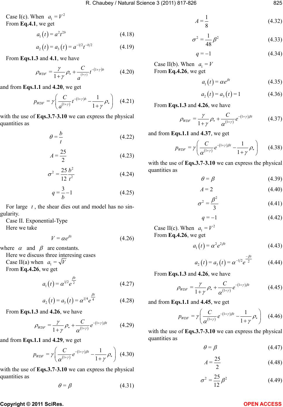
The Bianchi type-VIo universe has been considered
for a new equation of state for the Dark Energy compo-
nent of the universe (known as dark wet fluid). The solu-
tion has been obtained in quadrature form. The models
with constant deceleration parameter have been dis-
cussed in detail. The behaviour of the models for large
time have been analyzed.
REFERENCES
[1] Riess, A.G., et al. (1998) Observational evidence from
supernovae for an accelerating universe and cosmologi-
cal constant. Astronomical Journal, 116, 1009.
doi:10.1086/300499
[2] Perlmutter, S., et al. (1999) Measurements of Ω and 
from 42 high-redshift supernovae. Astrophysical Journal,
517, 565. doi:10.1086/307221
[3] Sahni, V. (2004) Dark matter and dark energy.
arXiv: astro-ph/0403324 (preprint).
[4] Ratra, B. and Peebles, P.J.E. (1988) Cosmological con-
sequences of a rolling homogeneous scalar field. Physi-
cal Review D, 37, 3406. doi:10.1103/PhysRevD.37.3406
[5] Caldwell, R.R., Dave, R. and Steinhardt, P.J. (1998)
Cosmological imprint of an energy component with gen-
eral equation of state. Physical Review Letters, 80, 1582.
doi:10.1103/PhysRevLett.80.1582
[6] Barreiro, T., Copeland, E.J. and Nunes, N.J. (2000)
Quintessence arinsing from exponential potentials. Phy-
sical Review D, 61, 127301.
doi:10.1103/PhysRevD.61.127301
[7] Armendariz-Picon, C., Damour, T. and Mukhanov, V.
(2001) K-inflation. Physics Letters B, 458, 209.
doi:10.1016/S0370-2693(99)00603-6
[8] Armendariz-Picon, C., Mukhanov, V. and Steinhardt, P.J.
(2001) Essentials of K-essence. Physical Review D, 63,
103510. doi:10.1103/PhysRevD.63.103510
[9] Gonzalez-Diaz, P.F. (2004) K-essential phantom energy:
Doomsday around the corner? Physics Letters B, 586, 1.
doi:10.1016/j.physletb.2003.12.077
[10] Caldwell, R.R. (2002) A phantom menace? cosmological
consequences of dark energy component with su-
per-negative equation of state. Physics Letters B, 545, 23.
doi:10.1016/S0370-2693(02)02589-3
[11] Carroll, S.M., Hoffman, M. and Trodden, M. (2003) Can
the dark energy equation-of-state parameter  be less
than −1? Physical Review D, 68, 023509.
doi:10.1103/PhysRevD.68.023509
[12] Elizalde, E., Nojiri, S. and Odintsov, S.D. (2004) Late-
time cosmology in a (phantom) scalar-tensor theory: Dark
energy and the cosmic speed up. Physical Review D, 70,
043539. doi:10.1103/PhysRevD.70.043539
[13] Freese, K. and Lewis, M. (2002) Cardassian expansion:
A model in which the universe is flat, matter dominated,
and accelerating. Physics Letters B, 540, 1.
doi:10.1016/S0370-2693(02)02122-6
[14] Gondolo, P. and Freese, K. (2003) Fluid interpretation of
cardassian expansion. Physical Review D, 68, 063509.
doi:10.1103/PhysRevD.68.063509
[15] Deffayet, C., Dvali, G.R. and Gabadadze, G. (2002) Ac-
celerated universe from gravity leaking to extra dimen-
sions. Physical Review D, 65, 044023.
doi:10.1103/PhysRevD.65.044023
[16] Dvali, G., Gabadadze, G. and Porrati, M. (2000) 4D grav-
ity on a brane in 5D minkowski space. Physics Letters B,
485, 208. doi:10.1016/S0370-2693(00)00669-9
[17] Dvali, G. and Turner, M.S. (2003) Dark energy as a
modification of the friedmann equation.
arXiv: astro-ph/ 0301510.
[18] Xanthopuolos, B.C. (1987) Perfect fluids satisfying a less
than extremely relativistic equation of state. Journal of
Mathematical Physics, 28, 905. doi:10.1063/1.527581
[19] Gorini, V., Kamenshchik, A., Moschella, U. and Pasquier,
V. (2004) The chaplygin gas as a model for dark energy.
arXiv: gr-qc/0403062 (preprint).
[20] Tait, P.G. (1888) The voyage of H.M.S. challenger. Lon-
don: H.M.S.O., 2, 1-73.
[21] Hayward, A.T.J. (1967) Compressibility equations for
liquids: A comprative study. British Journal of Applied
Physics, 18, 965.
doi:10.1088/0508-3443/18/7/312
[22] Chiba, T., Sugiyama, N. and Nakamura, T. (1998) Ob-
servational tests of X-matter models. Monthly Notices of
the Royal Astronomical Society, 301, 72.
doi:10.1046/j.1365-8711.1998.02012.x
[23] Holman, R. and Naidu, S. (2005) Dark energy from wet
dark fluid. arXiv: astro-ph/0408102 (preprint).
[24] Riess, A., et al., (2004) Type Ia supernova discoveries at
z > 1 from the hubble space telescope: Evidence for past
deceleration and constraint on dark energy evolution.
arXiv: astro-ph/0402512 (preprint).
[25] Bennett, C.L., et al., (2003) First-year Wilkinson Micro-
wave Anisotropy Probe (WMAP) obsevations: Prelimi-
nary maps and basic results. Astrophysical Journal Sup-
plement, 148, 1. doi:10.1086/345346
[26] Spergel, D.N. (2003) First-year Wilkinson Microwave
Anisotropy Probe (WMAP) obsevations: Determination
of cosmological parameters. Astrophysical Journal Sup-
plement, 148, 175. doi:10.1086/377226
[27] Tegmark, M., Hamilton, A.J.S. and Xu, Y.Z. (2002) The
power spectrum of galaxies in the 2 dF 100 k redshift
survey. MNRAS, 335, 887.
doi:10.1046/j.1365-8711.2002.05622.x
[28] Babichev, E., Dokuchaev, V. and Eroshenkos, Y. (2004)
Dark energy cosmology with generalized linear equation
of state. arXiv: astro-ph/0407190 (preprint).
[29] Singh, T. and Chaubey, R. (2008) Bianchi type-I universe
with wet dark fluid. Pramana—Journal of Physics, 71,
447-458.
[30] Chaubey, R. (2009) Bianchi type-V universe with wet
dark fluid. Astrophysics and Space Science, 321, 241-246.
doi:10.1007/s10509-009-0027-5
[31] Singh, T. and Chaubey, R. (2007) Bianchi type-V cos-
mological models with a viscous fluid and  -term.
Pramana—Journal of Physics, 68, 721-734.
[32] Singh, T. and Chaubey, R. (1998) Bianchi type-V and
VIo universes with dilaton and magnetic fields. Interna-
tional Journal of Modern Physics D, 15, 111.