Journal of Geographic Information System, 2011, 3, 334-344
doi:10.4236/jgis.2011.34031 Published Online October 2011 (http://www.SciRP.org/journal/jgis)
Moving towards Personalized Geospatial Queries
Giorgo s Mo untrakis1, Anthony Stefanidis2
1Department of Environmental Resources Engineering, State University of New York College of Environmental
Science and Forestry, Syracuse, USA
2Center for Geospatial Intelligence, Department of Geography & Geoinformation Science, George Mason University,
Fairfax, USA
Received July 3, 2011; revised August 8, 2011; accepted August 10, 2011
Abstract
Geospatial datasets are typically available as distributed collections contributed by various government or
commercial providers. Supporting the diverse needs of various users that may be accessing the same dataset
for different applications remains a challenging issue. In order to overcome this challenge there is a clear
need to develop the capabilities to take into account complicated patterns of preference describing user
and/or application particularities, and use these patterns to rank query results in terms of suitability. This pa-
per offers a demonstration on how intelligent systems can assist geospatial queries to improve retrieval ac-
curacy by customizing results based on preference patterns. We outline the particularities of the geospatial
domain and present our method and its application.
Keywords: Geospatial Databases, Geographic Information Systems, Geospatial Queries, Similarity Learning,
Preference Modeling, Adaptive Systems, Digital Government.
1. Introduction
Geospatial information enjoys an increasingly important
role in modern day societies, as it is used to support a
variety of activities ranging fro m long-term planning and
modeling, to emergency response and disaster manage-
ment. Geospatial datasets may be diverse in nature, rang-
ing from digital imagery and raster datasets to thematic
layers of geographic information systems (GIS), vector
data, and diverse sensor feeds. These datasets are col-
lected, stored, and distributed by a variety of federal (e.g.
the National Geospatial-Intelligence Agency—NGA),
state (e.g. various state GIS offices), or local (e.g. town
records) agencies. In addition to these authoritative data-
sets we are now witnessing the emergence of volunteered
and participatory GIS [1], with datasets collected and
contributed by non-profit organizations (e.g. Ushahidi)
or even individuals. Through advancements in sensor
technology, computer hardware, and software we have
now reached the point where massive amounts of diverse
types of geospatial datasets are integrated in distributed
petabyte-size archives.
As the applications that use geospatial datasets are
quite diverse, it is not rare to have the same dataset (e.g.
a specific GIS layer) accessed by different users to sup-
port diverse applications (e.g. location-based services
through cell phone apps), or decision-making activities
(e.g. land use modeling, crisis monitoring). In order to
support query-based information retrieval (IR), geospa-
tial datasets are indexed with metadata describing their
essential properties (e.g. date, scale, accuracy, resolution,
time, provider). Queries are typically performed by hav-
ing a user stating his/her preference in terms of these
metadata, e.g. “retrieve satellite images of Fukushima,
Japan after March 11 2011, with pixel resolution equal
to or better than 1 meter”. The suitability of available
datasets is the n evaluated u sing standard dista nce metrics
to compare them to the query request and rank them ac-
cording to their similarity to the query parameters [2].
However, standard IR approaches fail to capture pref-
erence differences among diverse users. For example, a
transportation expert and an emergency responder may
have different preference patterns as they aim to retrieve
satellite imagery depicting an area of interest at a specific
instance. In the above-provided example relating to the
Fukushima earthquake and subsequent tsunami, the
transportation expert would prefer the most recent image
available after the earthquake (e.g. from May, 2011), as
her task may be to update the road network maps and
capture the current state of transportation infrastructure

G. MOUNTRAKIS ET AL.335
in the area. On the other hand, the emergency responder
may be interested in imagery showing the tsunami at its
farthest location, before it started receding, to better as-
sess the full extent of the impact area. For this responder
the most recent imagery may therefore be of lesser value
than imagery captured one to two hours after the earth-
quake.
The above is a simple example that shows potential
variations in user-database interaction. Users that attempt
to access collections of geospatial datasets have diversi-
fied information needs, reflecting differences in the ex-
perience and/or task at hand. As the user community of
geospatial information is growing and becoming in-
creasingly more diverse, such preference variations are
becoming the norm rather than an exception. Standard IR
techniques fail to take into account such complex pref-
erence patterns. In order to overcome this shortcoming
we need to support the customization of user query exe-
cution by taking into account the particularities of a
user’s preferences. In this paper we present our approach
to model user preferences in geospatial applications in
order to improve the performance of geospatial queries.
Before we proceed to the specifics of our method, we
address trends in the generation, storage, and delivery of
geospatial information.
2. Geospatial Dataset Availability
Authoritative geospatial datasets have been traditionally
generated, used, and delivered by a variety of local, state,
and federal government agencies. They are typically
available as distributed collections through correspond-
ing portals.
A representative example of a federal collection of
geospatial datasets is the National Atlas (http://www.
natio nalatla s. go v/) , of fer in g m ap co ver a ge ac r oss t he US ,
with various themes (e.g. agricultural and transportation
data overlaid on basic maps). The National Geospa-
tial-Intelligence Agency (NGA, www.nga.mil) is offer-
ing access to charts and images. Users can access this
information through its Raster Roam interface. Users
can access a specific file either by selecting an area in a
map display, or by using geographic names in a gazet-
teer-like approach. Furthermore, the Federal Geographic
Data Committee (FGDC) (www.fgdc.gov) of the US
Geological Survey (USGS) offers a distributed discovery
mechanism comprising regional clearinghouses for digi-
tal geospatial dataset deli very. The Environmental Pro-
tection Agency (EPA) offers a wide variety of geospa-
tially-referenced information (e.g. water quality and haz-
ardous waste data), queried through a zip-code based
system (http://www.epa.gov/enviro/html/qmr.html). In an
effort to address the particular needs of disaster response,
government agencies have set up dedicated portals that
aggregate specific types of information. For example the
Geospatial Multi-Agency Coordination Group effort
(GeoMAC) (http://www.geomac.gov) aggregates fire-
related information (incl. fire perimeter, terrain, and
MODIS satellite datasets) across the continental United
States. The Natural Hazards Support System (NHSS)
( http://nhss.cr.usgs.gov) is another example of an inte-
grative portal, offering information on various natural
hazards, e.g. volcanic, earthquake, and flooding informa-
tion, together with satellite imagery. These federal-level
datasets are complemented by countless regional collec-
tions of geospatial datasets collected and distributed
through states, cities, and municipalities.
This early model of government-driven geospatial
dataset collection and ad ministration evol ved through the
proliferation of commercial remote sensing and geospa-
tial analysis endeavours. For example, TerraServer
(www.terraserver.com) is a collaboration of commercial
(Microsoft, Compaq) and federal (USGS) partners, that
offers a collection of digital imagery from numerous
providers, arranged by location (e.g. coordinates, city
name, street address, zip code), in various time instances.
USGS photography comprises few terabytes of data, and
is accessible through several host servers. Another nota-
ble commercialized collection of geospatial datasets is
Mapquest (www.mapquest.com), using maps of the
complete US in a variety of scales (e.g. 1:100,000,
1:25,000), 1-meter resolution aerial photography, and
detailed street maps. Probably the most popular com-
mercial implementation is the adaptation of Keyhole
technology to build Google Earth (earth.google.com),
aggregating a massive collection of satellite and field
data.
The latest evolution of geospatial dataset availability is
the on-going emergence of volunteered and participatory
geographic information (VGI). Crisis mapping is a par-
ticularly relevant example, with the aggregation of au-
thoritative datasets with contributed multimodal infor-
mation to capture the consequences and evolution of a
catastrophic situation [3,4]. Ushahidi (http://ushahidi.
com) and its utilization during the Haiti 2010 earthquake
disaster is by now a classic example of VGI at work. In
addition to these examples, where the general public is
contributing information, we also have services like
Google MapMaker (http://www.google.com/mapmaker),
where citizens are given the opportunity to perform in-
formation extraction tasks, like road centerline delinea-
tion, thus contributing directly geospatial information.
Thus we see that geospatial datasets are made avail-
able in numerous distributed collections of terabyte-sized
arc hives of go vernme nt, comme rcial, or non-pr ofit age n-
cies, each following established standards and specifica-

G. MOUNTRAKIS ET AL. 336
4) Based on user request an indexing mechanism is
used to return all potentially similar objects, in essence
filtering dissimilar ones to accelerate the retrieval proc-
ess. One filtering example is to temporary identifying all
buildings larger than 2000 m2 and ignores all other build-
ings.
tions in terms of a variety of parameters, including accu-
racy, format, metadata, scale, organization. Users access
these datasets through the corresponding agency portals,
either by browsing collections, or by forming meta-
data-based queries as mentioned in the previous section.
The challenge faced by applications employing geospa-
tial databases is to support the diverse needs of various
users that may be accessing the same dataset for differ-
ent applications. In order to do so we need to be able to
take into account the complicated patterns of preference
that correspond to a user and/or application, and use
these patterns to rank existing datasets in terms of suit-
ability.
5) On this filtered object collection a similarity algo-
rithm with properties extracte d from a knowledge base is
applied. The output is either a certain number of best
answers (e.g. 10 best datasets) or answers within a spe-
cific similarity range (e.g. higher than 80%). For further
information see section 6 of this paper.
6) The results are presented to the users to assess their
similarity accuracy. To help our paper readability, here are the definitions
of three important terms as presented within the context
of this paper: In the above information flow there are several areas of interest that the database community is working on.
Various disciplines are involved in the process and many
different approaches have been proposed. Specifically,
large distributed information source repositories are cre-
ated and issues related to storing and accessing these
databases are investigated. Ontologies are introduced to
compensate for different field descriptions, as well as
multi-node architectures and theoretical database models
to support them. Query languages and indexing mecha-
nisms for faster information retrieval are developed.
 Similarity refers to how appropriate is a given re-
sponse to a geospatial information request.
 Preference relates to users expressing their indi-
vidual suitability metrics for similarity.
 Similarity learnin g is the process of identifying and
expressing in mathematical terms user preference on
suitability.
3. Similarity in Geospatial Information
Our work concentrates on step five on the previous list.
The goal is to develop a similarity algorithm that will
rank the results in an accurate way. In order to do so,
when a user is performing a geospatial information re-
quest, some identification information of user prefer-
ences is forwarded to a knowledge base (dotted arrow on
the graph) and the appropriate similarity profile is ex-
tracted and incorporated in the query process.
Before we get into the specifics of our similarity learning
approach, let us first examine the information retrieval
process and the corresponding steps involved. Every
request for geospatial information involves a collection
of methods, some of which have been addressed exten-
sively in the literature and some others are newly inves-
tigated. In Figure 1, a schematic representation of the
query process is shown. The following steps take place: The current methodologies used for similarity assess-
ment of geospatial information have a common charac-
teristic: they are non-adaptable to specific user prefer-
ences, instead they are expressed as pre-defined similar-
ity measures and remain the same independently of
task/user requirements. Similarity calculation is per-
formed by storing geospatial information metadata as
points in the feature space and using a distance metric to
measure correlation to these points [5-7]. As mentioned
above, commonly used metadata information includes
expressions of resolution, accuracy, spatial extent, scale,
date, and source. Usually a Minkowskian p-distance [8]
is employed to define the similarity measure and is de-
fine d as:
1) Users request an information object from the data-
base (or more than one). For example a user may request
all buildings within a given area that are larger than 2000
m2 and within 1 km from a highway exit.
2) Their request is translated into a structured query
that the system understands and that is compatible with
the database collection. In this step the user-provided
information is matched to specific database fields and
content. For example, ontology may be used to match the
query for “buildings”, a non-existent term in the database,
to “single-family detached houses”, an existent field in
the database and therefore resolve ambiguity.
3) A query language is used as a mediator between
user and database. This step is essential to convert user
preferences into an automated executable code for in-
formation retrieval. One predominant example of such
programming language is Structured Query Language
(SQL).



1
1
(,) p
p n
pi
i
Lxyx y


i
For p = 2 we have the traditional Euclidean distance
metric. If p = 1 then the Minko wskian distance expresses
the Manhattan distance func tion. Another funct ion is the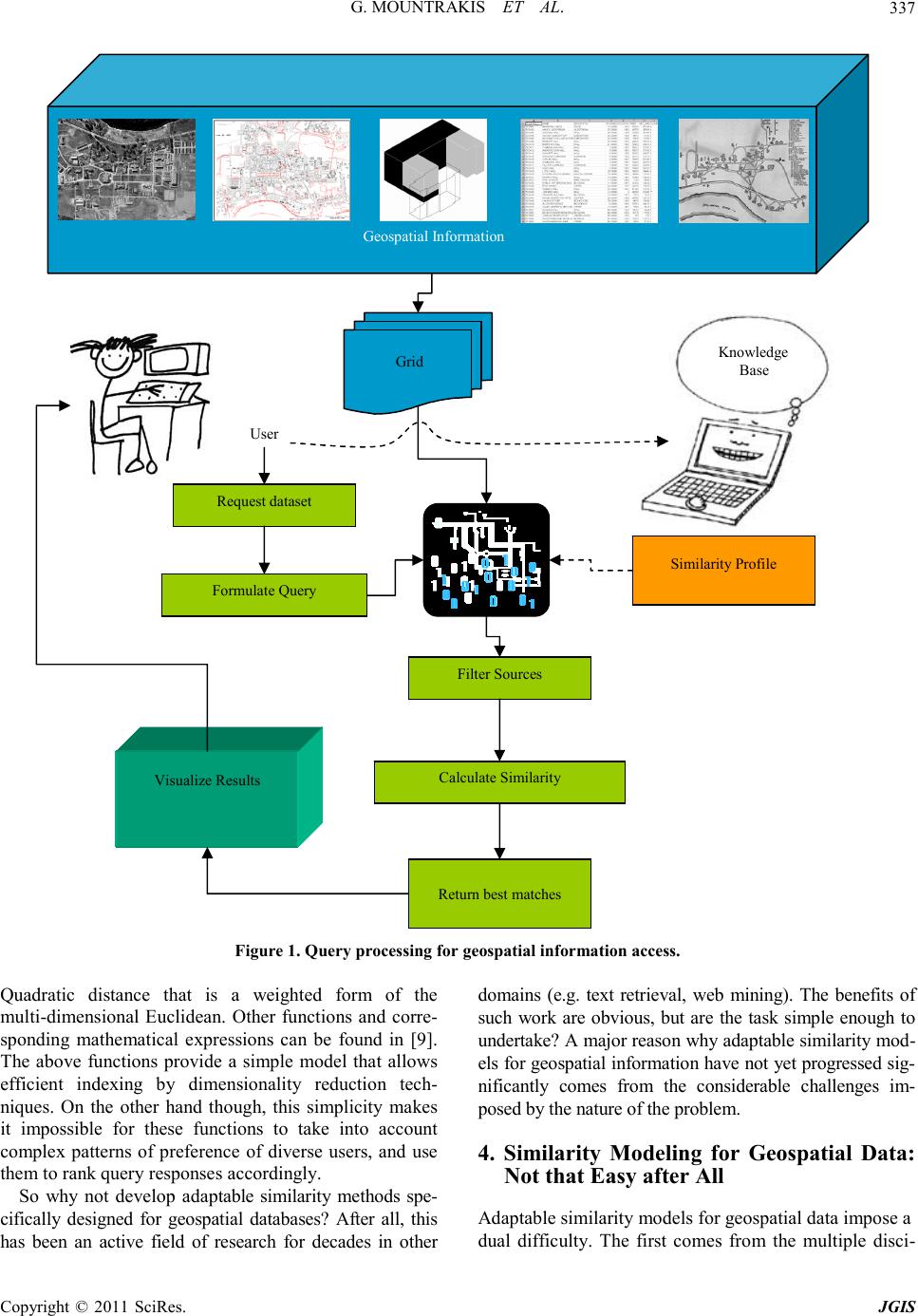

G. MOUNTRAKIS ET AL.337
Geospatial Information
Figure 1. Query processi ng for geospatial informati on access.
Quadratic distance that is a weighted form of the
multi-dimensional Euclidean. Other functions and corre-
sponding mathematical expressions can be found in [9].
The above functions provide a simple model that allows
efficient indexing by dimensionality reduction tech-
niques. On the other hand though, this simplicity makes
it impossible for these functions to take into account
complex patterns of preference of diverse users, and use
them to rank query responses accordingly.
So why not develop adaptable similarity methods spe-
cifically designed for geospatial databases? After all, this
has been an active field of research for decades in other
domains (e.g. text retrieval, web mining). The benefits of
such work are obvious, but are the task simple enough to
undertake? A major reason why adaptable similarit y mod-
els for geospatia l informatio n have not yet progressed s ig-
nificantly comes from the considerable challenges im-
posed by the nature of the problem .
4. Similarity Modeling for Geospatial Data:
Not that Easy after All
Adaptable similarity models for geospatial data impose a
dual difficulty. The first comes from the multiple disci-
Fil ter S ource s
User
Request dataset
Similarity Profile
Calculate Simi larity
Return best ma tches
Formulate Query
Knowledge
Base
Visualize Results
Grid

G. MOUNTRAKIS ET AL. 338
plines involved in the similarity learning task and it is
not unique to geospatial datasets. The second difficulty
rises from the particularities of the geospatial domain
and corresponding user needs. This uniqueness of the
geospatial domain is the focus of our attention.
4.1. The Interdisciplinary Nature of Similarity
Learning
Three general areas of research have been suggested in
[10], namely psychology, data mining and machine
learning. Briefly discussed here, the psychologists have
concentrated on the human understanding and expression
of similarity. Their research verifies that there is an ob-
jective parameter (i.e. user dependent), which has to be
addressed for successful similarity modeling. Building
on that, several tasks from the data mining field can be
borrowed to accomplish our goal, tasks such as classifi-
cation, regression, time series analysis and others. As
expected, similarity learning naturally also falls under
the general category of machine learning methods. The
influence from multiple disciplines such as statistics,
databases and artificial intelligence in machine learning
is well-documented in the literature. From the similarity
learning perspective an important distinction of machine
learning algorithms is between supervised and unsuper-
vised methods. Since most similarity learning algorithms
learn from example, in other words they need a supervi-
sor (teacher) to provide them some reference output val-
ues, they belong in the supervised category.
4.2. Particular it i es of the G e osp atial Do main
Similarity learning in database queries is intrinsically
connected with the data types stored. Geospatial data
have important differences to online analytical process-
ing data, general multi-dimensional data, traditio nal rela-
tional data or transactional data [11]. This uniqueness is
partially attributed to the integrative nature of GIS. Many
of the issues arise from the fact that geographic data span
a wide range of perspectives and interests from the social
to the physical aspects of the problem [12]. This mixture
of perspectives coupled with the growing infrastructure
for gathering information pose the following challenges:
1) Diverse data types. The wide variety of digital geo-
graphic data imposes a number of constraints/demands to
similarity learning algorithms. Distributed datasets are
becoming increasingly prevalent and important as a source
of geographically referenced data [13] and thus tend to
comprise a variety of geo-referenced multimedia data
types, such as still and video imagery, text, graphics, and
ev en au d io and anim at ion s [14] .
2) Dimensiona lity g ro uping and depe ndencie s. Geo-
spatial databases tend to be high-dimensional, as for
example location information is accompanied by radio-
metric content, elevation data, ownership information,
and temporal records. It is important to note that among
these multiple dimensions we can recognize groups that
are highly related among themselves, but remain quite
different from other groups. For example, there exists a
high conceptual affinity among the three spatial dimen-
sions (x,y,z) as they are represented by similar structures
and often have comparable values, while there is an ob-
vious lack of such affinity among them and an alphanu-
meric ownership record. Accordingly, dimensions tend
to be grouped together in conceptual features (e.g. spatial
information, thematic attributes).
However, regardless of conceptual affinity, heteroge-
neous features may display high dependency among
them (e.g. space and time). This dependency needs to be
exploited when querying a database in order to recognize
for example complex spatiotemporal events and patterns.
Querying space and time separately would fail to ade-
quately address this inherent spatiotemporal complexity.
Similarly, the radiometric content of satellite imagery
may be highly correlated to sensor information. This
grouping of dimensions and the need to exploit
cross-grouping dependencies is another issue that differ-
entiates geospatial databases from other high-dimensio-
nal o nes.
3) Data volume. Like many disciplines where learn-
ing algorithms are applied, GIS is rich in data. In addi-
tion to traditionall y considered geospatial datab ases (e.g.
maps, photographs), numerous other databases (e.g.
consumer, medical, and financial records) are now incor-
porating spatial and temporal attributes and hence offer
the possibility of discoverin g or confirming geographical
knowledge [15]. As mentioned above, geospatial dataset
collections are now terabyte-sized, and traditional re-
trieval methods have a hard time to keeping up. Further-
more, maintaining and evaluating these large amounts of
information is a major challenge, leading to frequent oc-
currence of incomplete or missing data.
4) Complexities due to loca l variation. Earth systems
are so intrinsically interconnected that it is difficult to
isolate an analysis conducted on some part of a system
from the affects of other unmodeled aspects [8]. This
translates into potential generalization problems of simi-
larity algorithms. Measured geographic attributes often
exhibit the seemingly contradictory properties of spatial
correlation and spatial heterogeneity. The former (corre-
lation) refers to the tendency of attributes at some loca-
tions in space to be related, also known as Tobler’s first
law of geography [16]: “Everything is related to every-
thing else but nearby things are more related than distant
things”. However, and despite the effect of spatial corre-

G. MOUNTRAKIS ET AL.339
lation on the major trends of spatial information, geo-
graphic phenomena are often highly localized. Spatial
heterogeneity describes this non-stationarity of most
geographic processes, and expresses the fact that global
parameters do not necessarily describe well the localized
nature of some geographical phenomena.
5) Granularity. In most non-geographic domains,
data objects are meaningfully represented discretely
within the information space without losing important
properties [17]. But this does not seem to extend to geo-
graphic objects [18]: size, shape and boundaries can af-
fect geographic processes, therefore generalization can-
not be achieved without information loss in both raster
and vector representations. Scales and granularities for
measuring time are also complex, preventing a simple
“dimensioning up” of space to include time. Moreover
micro data, observations on individual observational
units, might not always be accessible, e.g. due to dis-
semination, confidentiality or cost constraints. Macro
data (aggregates of micro data) are used instead. Exam-
ples of macro data include counts, frequencies, sums,
averages and other statistics characterizing micro data.
5. Geospatial User Profiles
5.1. Motivation
Until now we defined desired characteristics for a simi-
larity learning algorithm. Similarity is typically calcu-
lated by comparing a stored set of values to the ones the
users query for. First each query value (attribute) is
compared to the corresponding stored one, for example
the time of a stored aerial photograph to the correspond-
ing query value for time, the scale of the stored aerial
photograph to the query and so on for every requested
attribute. Then results from this comparison expressing
similarity within every attribute (similarity in time, scale,
etc) are aggregated to provide an overall similarity met-
ric, a metric showing the overall similarity between the
query and the stored aerial photograph based on these
individual metrics from every attribute.
Existing methodologies concentrate on multi-attribute
(i.e. multi-dimensional) si milarity aggregation to provide
an overall similarity metric. In some cases though prob-
lem complexity relies o n the si milarity calculation within
each dimension separately rather than on their combined
aggregation. This is frequently the case when querying
for GIS datasets. The information retrieval process might
fail because the individual similarity metrics in every
dimension may not be able to capture user similarity
preferences.
A common example of such similarity preference in
GIS is when asymmetric, non-linear user behavior is
exhibited during the direct comparison of attributes. For
example, let us consider a geospatial database and a user
request for an aerial image of specific ground pixel size
for building extraction. User interest decreases gradually
(but not necessarily linearly) as pixel size increases to the
degree that buildings would not be identifiable. Further-
more, the user may have cost considerations (e.g. cost,
storage and processing time) associated with a higher
resolution acquisitio n. This tr anslates to a similarity rela-
tion that can also be non-linear as resolution improves.
So it is easily understood that we need asymmetrical,
non-linear relations to model user preference within each
attribute comparison. Thus, in geospatial queries user
preferences may be significantly more complex than
general queries (e.g. text queries), while the diversity of
users and applications is further emphasizing the need
for efficient modeling. Therefore, modeling user similar-
ity preference within each attribute can substantially help
geospatial queries. Motivated by these observations, the
focus of our work is to investigate the application of
complex functions for user preference within each attrib-
ute. The integration of similarity results from multiple
attributes is part of our future work.
5.2. A User Preference-Based Approach
In order to adapt similarity models to user preferences
we developed a relevance feedback algorithm. Users are
presented with a variety of pairs of requested and re-
turned values and are asked to provide a preference met-
ric for each pair. The corresponding training dataset is
created and used as input for our preference learning
method. Figure 2 shows a typical training session, where
the user is given the Query (X axis), and Database value
(Y axis) and is requested to provide a similarity assess-
ment of these two.
The result corresponds to the Similarity value (Z axis).
The problem can easily be seen as a surface-fitting one,
Figure 2. Training example.

G. MOUNTRAKIS ET AL. 340
where it is attempted to substitute the provided three-
dimensional points with a surface (function). For training
several preference models are used of as expressed
thro ugh a varie ty of fuzz y member ship f unctio ns (FMFs) .
The approach is simple yet effective: gradually increase
the complexity of the underlying FMF until an accept-
able solution is reached. The process begins by interpo-
lating a set of planes to the training dataset [19]. We
examine the resulting accuracy and if it is within the
predefined specifications we end the process. These pre-
defined specifications are in essence thresholds describ-
ing the maximum acceptable error between the interpo-
lated functions and the training points. They can be pre-
set by the database designer or adjusted in real-time by
the user. If the results are not within these thresholds, we
examine the obtained plane parameters. This analysis
leads to a decision whether similarity is dependent on the
query value, their difference metric or the actual database
and query values. We continue by interpolating two sig-
moidal functions whose initial approximations are calcu-
lated from the plane properties. If required accuracy is
not achieved, we provide further modeling capabilities
by parameterizing further the FMFs parameters. At the
last stage we obtain the best possible set of FMFs that
express user preference as presented through the training
set. If accuracy is not yet achieved, we trigger a neural
network process to correct local errors. More information
on the training mechanism and the corresponding mod-
eling capabilities can be found in [19].
After the best possible set of functions is identified,
the mathematical properties of the model are stored in
the form of a profile. This profile can also contain a User
ID, and potentially comments/keywords that will allow
usability of the same profile from other users to avoid
retraining the system. For example, such keywords might
be general such as “Photogrammetrist” o r “Biologist”, or
more task-specific such as “Airplane feature extraction”,
“Wetland evaluation”.
To further demonstrate the app licability of the method
a representative example is presented below for a cadas-
tre/real estate application. More specifically, this sce-
nario investigates user preference of a geospatial attrib-
ute expressing parcel value per square meter. The func-
tion is composed of two sub-functions, each one applica-
ble in half of the input space (e.g. Xq > Xdb) to compen-
sate for asymmetrical cases. A result of this trained func-
tion can be seen in Figure 3.
Figure 4 shows similarity isolines (0% to 100% at the
graph floor) of the surface from Figure 3, in essence
combinations of query and database values that would
result in the same similarity value. In addition, two spe-
cific user queries are examined through the two slices,
for parcel value per square meter (PVSM) of $500/m2 (in
orange) and $3000/m2 (in green). Examination of these
two sections leads to two remarks:
1) The left side of each of the two sections examines
the case where the returned PVSM value (Xdb) is smaller
than the query PVSM value (Xq). Here the method is able
to express the gradual decrease of user’s interest. Note in
Figure 4 how user flexibility increases as the PVSM
query value becomes larger.
2) The right side of each of the two sections examines
the case where the returned PVSM value (Xdb) is larger
than the query PVSM value (Xq). From the two sections
Figure 3. Example of a user preference function.

G. MOUNTRAKIS ET AL.341
Figure 4. Contour plot and query examples of this preference function.
it is evident that a s the query PVSM value (Xq) increases
so does the user flexibility on the obtained results. More
specifically, when users request the retrieval of database
objects with $500/m2 PVSM they are less flexible in ac-
cepting larger values than when querying for a $3000/m2
one.
6. Using Profiles in Queries
In order to demonstrate the applicability of our method,
let us consider the following scenario. The City of
Tempe had cameras installed to monitor its downtown
area. Numerous city agencies use this information for
their various needs. For example, let’s consider that im-
agery from these cameras is accessed by both the Police
and Transportation Departments. Let’s also assume that
they perform similar queries, using last year’s New
Year’s Eve imagery database to train personnel in an-
ticipation of this year’s celebrations. They are interested
in recovering an image of the downtown area at 12 mid-
night, to get a snapshot of the situation, so they form a
query to express this request. Even though they form the
same query, the execution of this query proceeds differ-
ently for these two agencies, making use of their prefer-
ences as they are expressed through corresponding pro-
files. Algorithm training is performed based on estab-
lished similarity preferences, and the corresponding
similarity profiles are shown in Figures 6 and 7 for the
Police and Transportation Departments, respectively. For
comparison we also present a generic profile in Figure 5.
By using these different profiles in the query process-
ing it is feasible to rank available imagery differently,
taking i nto acco unt thei r diffe rent ne ed s. For e xample , th e
Police profile has the following main characteristics:
 The time interval 11 pm - 12 am is of prime impor-
tance, as this is the instance with the highest crowd
concen t ration a nd o vera ll a c t i vit y.
 After 12 midnight interest begins dropping, as people
start leaving , but remains high u ntil 3 am.
On the other hand, the Transportation profile has some
other characteristics:
 Its peak is around 12 am, when people (potentially
into xicated) start leaving t he area, posing a highe r risk
of accidents .
 Early on, interest is increasing as we move from the
standard t raffic pa tterns of 9 pm to higher tr affic load s
by 10:45 pm.
 Intere st drops between 10 :45 pm and 11 :15 p m, as by
that ti me peop le ha ve alre ady arr i ved, and t hus vehi cle
traffic is limited. It starts picking up again after 11:30
pm as few people may be leaving earlier.
A sample of 5 images has been ranked, to demonstrate
the effects of user preferences. This is shown in Figure 8.
For example, that imagery from 11:20 pm is ranked first
for the police department, even though it deviates from
the query request (midnight) by 40 minutes, when there
is an image with only 15 minutes away from the query
time (12:15 am). However, for the above mentioned rea-
sons the 11:20 pm is more suitable for this department’s
needs than the 12:15 am snapshot. Other rankings have
similar explanations based on the above mentioned spe-
cial preference characteristics as expressed through the
corresponding profile. It is obvious that generic profiles
could not express such diverse similarity preference pat

G. MOUNTRAKIS ET AL. 342
Figure 5. Generic similarity profile.
Figure 6. Police surveillance similarity profile.
terns, limiting the effectiveness of query-based informa-
tion retrieval.
7. Conclusions
Geospatial datasets are becoming increasingly multifunc-
tional, as different users may be using the same dataset
for different applications. Accordingly, the successful
functional integration such datasets in federated geospa-
tial databases depends upon the ability to meet the needs
of expanding and diverse user communities. Therefore,
the development of efficient information retrieval meth-
ods to support the diverse and complicated preference
patterns of different users and/or applications is a crucial
task for the geoinformatics community.
In this paper we presented an approach to meet this
Time
Figure 7. Traffic monito ring similarity profile.
need through the introduction of user profiles of varying
complexity to model the requirements of different classes
of users when attempting to recover specific geoinforma-
tion. Intelligent systems can assist geospatial queries to
improve retrieval accuracy by customizing results based
on preference patterns. The profiles may vary in their
complexity, thus capturing the underlying preference in-
tricacies that differentiate user groups (e.g. the needs of a
transportation expert versus the ones of a police author-
ity).
As presented in this paper, our method emphasizes
preference modeling within specific attributes (e.g. pref-
erences in time, scale, resolution). Our future plans in-
clude the extension of this work to aggregate these indi-
vidual components into composite multidimensional user
profiles. Depending on the application range of a specific
government agency, these composite profiles may reflect
preferences of a single analyst or of a broader unit with a
specific mission and modus operandi.
While user preference profiles were introduced in this
paper as a tool to support information retrieval tasks,
they also encapsulate operational knowledge: they are
expressions of a user’s typical tasks and processes. Ac-
cordingly, we can recognize a very intriguing indirect
benefit of our approach, namely the ability to identify
similarities in user communities that may be operation-
ally different. For example, by comparing user profiles
between groups of analysts from an environmental and
an emergency response agency we may reach the con-
clusion that they have comparable preferences and tend
to perform similar tasks. This information can be used
for operational alignments across different units/agencies.
Furthermore, preference profiles may be used to priori-
tize data collection and information acquisition needs.
Types of datasets that exhibit high similarity preference

G. MOUNTRAKIS ET AL. 343
Figure 8. Effects of profiles on geospatial query results (images from www.tempe.gov).
R Ra an nk ki in ng g R Re es su ul lt ts s
1
1. .
2
2. .
3
3. .
4
4. .
5
5. .
9
9: :4 45 5p pm m
1
1: :3 30 0a am m
1
12 2: :4 45 5a am m
1
12 2: :1 15 5a am m
Generic Profile Police Profile Transportation Profile
1
1. .
2 2. .
3 3. .
4
4. .
5 5. .
9
9: :4 45 5p pm m
1
1: :3 30 0a am m
1 12 2: :4 45 5a am m
1 12 2: :1 15 5a am m
1
1. .
2 2. .
3 3. .
4
4. .
5 5. .
9
9: :4 45 5p pm m
1
1: :3 30 0a am m
1 12 2: :4 45 5a am m
1
12 2: :1 15 5a am m
1 11 1: :2 20 0p pm m
1
11 1: :2 20 0p pm m
1
11 1: :2 20 0p pm m

G. MOUNTRAKIS ET AL. 344
across numerous profiles should be updated more fre-
quently than others with lower priority. Combined with
the above mentioned capability to identify across agen-
cies clusters of users with similar needs and preferences,
this would provide crucial support for the reconfiguration
of government resources to best address evolving needs
and emerging challenges.
8. References
[1] M. F. Goodchild, “Citizens as Sensors: The World of
Volunteered Geography,” GeoJournal, Vol. 69, No. 4,
2007, pp . 211-221. doi:10.1007/s10708-007-9111-y
[2] V. M. Megler and D. Maier, “Finding Haystacks with
Needles: Ranked Search for Data Using Geospatial and
Temporal Characteristics. Scientific and Statistical Data-
base Management,” Scientific and Statistical Database
Management, Vol. 6809, 2011, p p. 55-72.
doi:10.1007/978-3-642-22351-8_4
[3] D. Sui, “The Wikification of GIS and Its Consequences:
Or Angelina Jolie’s New Tattoo and the Future of GIS,”
Computers, Environment, and Urban Systems, Vol. 32,
No. 1, 2008, pp. 1-5.
doi:10.1016/j.compenvurbsys.2007.12.001
[4] S. Liu and A. Iacucci, “Crisis Map Mashups in a Partici-
patory Age,” American Congress on Surveying a nd Map -
ping Bulletin, 2010, pp. 10-14.
[5] D. W. Aha, D. F. Kibler and M. K. Albert, “Instance-
Based Learning Algorithms,” Machine Learning, Vol. 6,
No. 1, 1991, pp. 37-66 . doi:10.1007/BF00153759
[6] W. Cheng and E. Huellermeller, “Combining Instance-
Based Learning and Logistic Regression for Multilable
Classification,” Machine Learning, Vol. 76, No. 2-3,
2009, pp . 211-225. doi:10.1007/s10994-009-5127-5
[7] P. Cunningham, “A Taxonomy of Similarity Mechanisms
for Case-Based Reasoning,” IEEE Transactions on
Knowledge and Data Engineering, Vol. 21, No. 11, 2009,
pp. 1532 -1543. doi:10.1109/TKDE.2008.227
[8] B. Batchelor, “Pattern Recognition: Ideas in Practice,”
New York Plenum Press, New York, 1978, pp. 71-72.
[9] D. R. Wilson and T. R. Martinez, “An Integrated In-
stance-Based Learning Algorithm,” Computational Intel-
ligence, Vol. 16, No. 1, 2000, pp. 1-2 8.
doi:10.1111/0824-7935.00103
[10] G. Mountrakis, P. Agouris and A. Stefanidis, “Similarity
Learning in GIS: An Overview of Definitions, Prerequi-
sites and Challenges,” In: M. Vassilakopoulos, A. Papa-
dopoulos and Y. Manolopoulos, Eds., Spatial Databases:
Technologies, Techniques and Trends, Idea Group Inc.,
Calgary, 2004, pp. 294-321.
doi:10.4018/978-1-59140-387-6.ch013
[11] D. Gunopulos, “Data Mining Techniques for Geospatial
Applications,” National Academies White Paper, 2001 .
[12] M. Gahegan, “Intersection of Geospatial Information and
Information Technology,” National Academies White
Paper, 20 01.
[13] National Research Council, “Distributed Geolibraries:
Spatial Information Resources,” National Academy Press.
Washington, DC, 1999.
[14] A. S. Camara and J. Raper, “Spatial Multimedia and Vir-
tual Reality,” Taylor & Francis, London , 19 99.
[15] H. J. Miller and J. Han, “Geographic Data Mining and
Knowledge Discovery: An Overview,” In: H. J. Miller
and J. Han, Eds., Geographic Data Mining and Knowl-
edge Discovery, Taylor and Francis, London, 2001.
doi:10.4324/9780203468029_chapter_1
[16] W. Tobler, “Cellular Geography,” In: S. Gale and G.
Olsson, Eds., Philosophy in Geography, Reidel, Dortrecht,
1979, pp . 379-38 6.
[17] M. Yuan, B. Buttenfield, M. Gahegan and H. Miller,
“Geospatial Data Mining and Knowledge Discovery,” A
UCGIS White Paper on Emergent Research Themes,
2001.
http://www.ucgis.org/emerging/
[18] J. Lin, Y. Fang, W. Zhang and Z. Huang, “Fundamental
Aspects of Access Control for Geospatial Data,” Interna-
tional Journal of Digital Earth, Vol. 2, No. 3, 2009, pp.
275-289. doi:10.1080/17538940902818329
[19] G. Mountrakis and P. Agouris, “Learning Similarity with
Fuzzy Functions of Adaptable Complexity. 8th Interna-
tional Symposium on Spatial and Temporal Databases,”
Lecture No tes in Comput er Science, Vol. 2750, 2003, pp.
412-429. doi:10.1007/978-3-540-45072-6_24