Technology and Investment
Vol.1 No.1(2010), Article ID:1333,8 pages DOI:10.4236/ti.2010.11008
Hybrid Decision Models in Non-Proportional Reinsurance
Department of Business Statistics, Friedrich-Schiller-University Jena, Germany
E-mail: maik.wagner@uni-jena.de
Received November 18, 2009; revised December 14, 2009; accepted December 17, 2009
Keywords: Insurance; Optimization; Risk; Decision Analysis
Abstract
Over the past years, risk measurement and therewith risk measures became more and more important in economics. While in the past risk measures were already adopted at the deposit of credit and shareholders equity, the approach now generates two hybrid decision models and applies them to the reinsurance business. The two introduced models implement a convex combination of risk measures and with it provide the possibility of modelling risk attitudes. By doing that, for the two hybrid decision models on the one hand can be shown, which risk attitude leads to the acceptance of a reinsurance contract and on the other hand, a deductible of which height an insurer is willing to undertake. Hence the possibility exists to identify the risk attitude of an insurer. In return, due to the knowledge of risk attitudes, under similar conditions the possibility arises to establish recommendations about the extent of the deductible at reinsurance contracts.
1. Introduction
The application of risk measures gains more and more importance. These measures can be applied on the one hand in the determination of the deposit of equity capital and on the other hand in the modelling of decision models considering the risk attitude. First of all, in Section 2 a short insight into the topic reinsurance should be given, in order to introduce subsequently the profit function of an insurer for a non-proportional reinsurance contract. In Section 3 two complementary decision principles will be introduced. These use a hybrid preference functional for the determination of the deductible. With the help of this the optimal deductible of an insurer can be determined depending on the insurers risk attitude (see Section 4). The interpretation of the results follows in Section 5 and will be completed by a prospect in Section 6. Hence the aim of the article is to show possibilities of integrating risk attitudes into the determination of deductibles.
2. Non-Proportional Reinsurance
An insurer uses a reinsurance [1–3] for risk limitation and risk diversification of its compulsory treaty indemnity with its private customer. Thereby the aim of a reinsurance is to replace a part of the assumed ambiguous costs of the losses by fixed costs. These fixed costs represent the recompense of the reinsurance, the so-called reinsurance premium. Hence the reduction of the risk charge plays a central role for the insurer.
In this process reinsurance has two fundamental tasks: First, to restrain the annual variation of the loss burden of the insurer and second, to ensure the solvency of the insurance company in the extreme event of loss. Consequently the violation of the solvency [4] is the highest risk, which the insurer wants to avoid.
Reinsurance contracts can be distinguished in the reinsurance form and hence in the limitation of the obligation or voluntariness of the acceptance of risks, but also in their type. The distribution of risk is crucial for this differentiation between the insurer and the reinsurer. The risk is divided between the parties either in a proportional or non-proportional way [5,6]. In the following the focus is only on the non-proportional reinsurance.
The non-proportional reinsurance is characterized by a liability of the reinsurer which is only influenced by the amount of loss. This implies in connection of the arrangement of the contract, that the reinsurer only contributes to the loss in case the determined limit of loss is exceeded. This limit of loss is called deductible. The loss burden undertaken by the reinsurer is called reinsurance loss. It is necessary that the reinsurance loss


whereas d is the deductible and X the loss that evolves from the private customer business. The loss describes a random variable with a distribution function and the corresponding density f. This density is zero for negative values, due to the non-existence of negative losses.
In return for the acquired reinsurance protection the insurer pays the reinsurance premium  The basic structure of such a premium contains the expected reinsurance loss and an additional profit mark-on. The profit mark-on can refer to the expected reinsurance loss on the one hand and to the variance or to the standard deviation on the other hand [7]. In the following the premium is applied with a profit mark-on, which is linked to the expected reinsurance loss.
Definition 1
 is the expected reinsurance loss and g the profit mark-on of the reinsurer with
 . Then
  is called reinsurance premium.
Additionally to the incomes and costs from the reinsurance business the reinsurer possesses the insurance premium Pr from the private customer business minus the loss X. Additionally the insurer has the costs of operation B. Consequently the profit function of an insurer has the following form

an insurer has the choice between different decision principles. For each decision principle a preference functional, modelling its behaviour, exists. In this process the aim of an insurer is to maximize its profit function in reference to the deductible.
3. Decision Principles
A situation is identified as decision under risk [8,9] in case the possible entry scenarios as well as their entry probabilities are known. Consequently this case applies to an insurer, as the cedent knows the loss distribution from historical data and hence the insurer can estimate the possible loss as well as its probability.
In the following, two hybrid models are introduced and applied to the reinsurance problem. Both decision models represent a weighting between expected value and conditional expected value. The first preference functional uses the Conditional Value at Risk (the lower conditional expected value) and the second preference functional the upper conditional expected value of the target function.
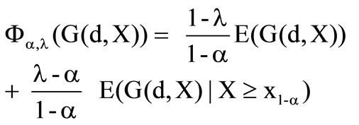
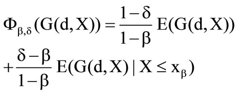
The preference functionals have the following form

and
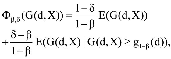
whereas  and
and  are the risk parameters of the first preference functional and
  and
and  are the risk parameters of the second preference functional with
  and
and . It is necessary that
 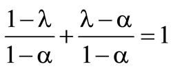 and
and 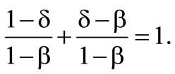 Furthermore
  is the a–quantile of the profit in the first and
  is the
  quantile of the profit in the second functional. Both preference functionals can be applied amongst others in the Newsvendor problem [10,11] with risk preferences [12,13].
In the Newsvendor model a trader wants to sell a product at the price p. However the product can only be sold within one time period. The trader buys the product at price c and in case of not selling can return it at the price of z. The analogy between the News-vendor and the reinsurance model is represented in Poser, Wagner [14].
Both preference functionals represent risk neutrality in case of equality of their risk parameters. In this case both functionals are equal the expected profit. In case  the lower expected value has a positive influence on the preference functional and represents risk aversion. Analogical in the second functional the upper expected value has a positive influence for
  and consequently reflects risk taking. In cases
  and
and  the lower and upper expected value is integrated negatively and represents risk taking for the first decision functional and risk aversion for the second one. It should be present that the complementary preference functionals have the same results.
The two following questions shall be clarified for the two introduced preference functionals:
1) At which risk attitude the insurer decides in favour of the reinsurance?
2) If the insurer decides in favour of the reinsurance, which level of the deductible is preferred?
4. Determination of the Deductible
In this section the deductible is determined with the help of two preference functionals depending on the risk attitude of a decision maker. The profit function is dependent on the loss while the lower and upper expected value comprise the profit quantile.
From Chart 1 can be noticed, that the  low-
low-
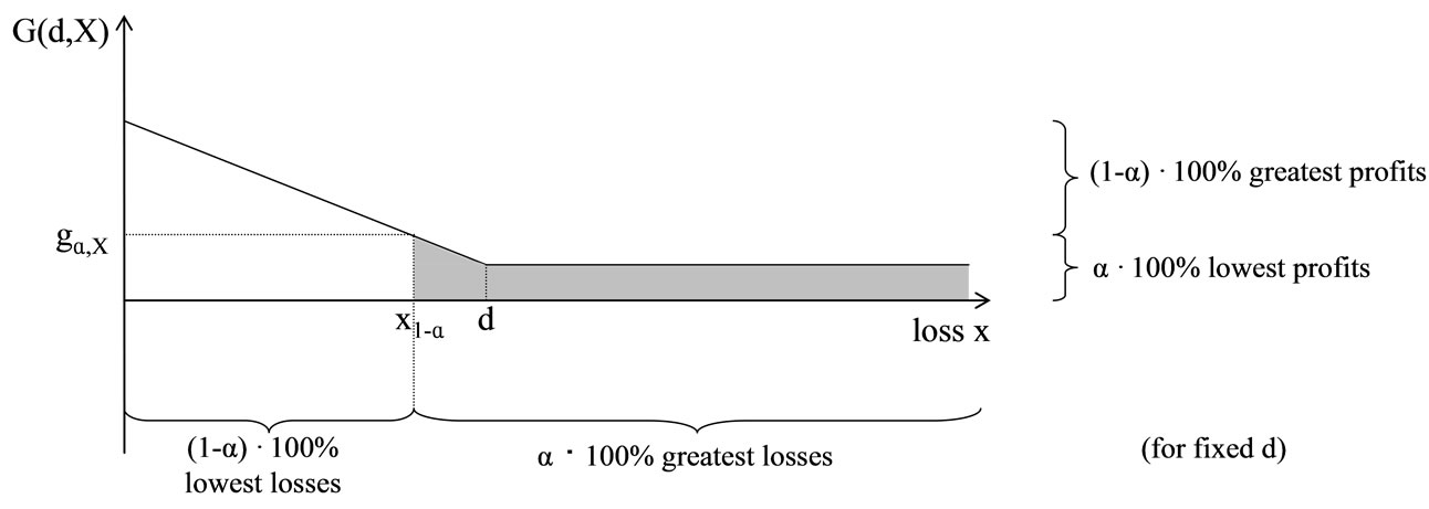
Chart 1. Profit function of the insurer with α-profit quantile.
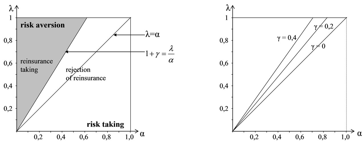
Chart 2. Risk preference space for the preference functional .
.
est profits are realized with the  greatest losses. Consequently
  of the losses are located below the loss quantile. Consequently it is the
  -loss quantile.
Hence the following equation applies

whereas  indicates the loss quantile. Analogical the
  greatest profits1 appear at the
  lowest losses.
  of the losses are located below the b-loss quantile. Hence the following applies
 )
)
whereas  characterizes the b-loss quantile. Hence it is possible to maximize the two preference functionals. The two following theorems verbalize this.
Theorem 1
Let  be the profit function of an insurer and
its objective function. Then the maximizing problem  has the following implicit solution

with  and
and .2
.2
Theorem 2
Let  be the profit function of an insurer and
its objective function. Then this maximizing problem  has the following implicit solution

with  and
and  [16].
[16].
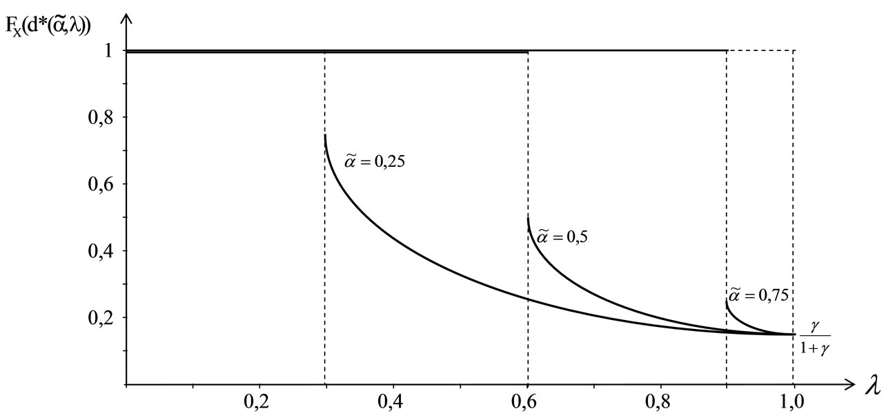
Chart 3.  for a given
 .
.
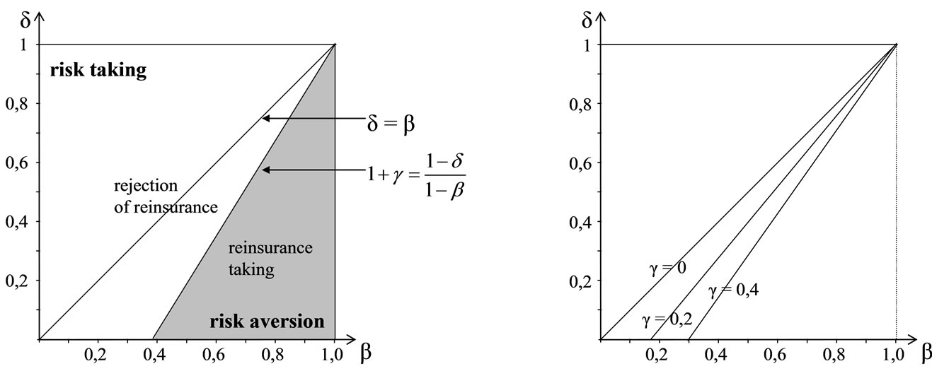
Chart 4. Risk preference space for .
.
5. Interpretation
At first the risk preference space for the preference functional  is examined. This one is illustrated by the left figure of the Chart 2. The space is splitted into two halves by the angle bisector. The surface above the angle bisector
  contains all
  combinations for risk aversion and below
  all combinations for risk taking. The angle bisector
  itself is the combination for risk neutrality.
Furthermore within this figure appears the border between the optimal solutions . The value of the distribution at the optimal deductible below that border thereby is
  and above
The conclusion can be drawn, that the insurer with chooses a deductible to the extent of the greatest losses. This implies, that the insurer wants to bear every occurred loss himself. In this case the cedent rejects the reinsurance. In the case
  the distribution of the optimal deductible fulfils

That implies, that the insurer intends to take the reinsurance. At the border  the insurer is indifferent between the optimal solutions.
The right figure of Chart 2 illustrates the changing of the border between contract taking and rejection depending on the profit mark-on of the reinsurer. The border moves in an area of higher risk aversion for a higher profit mark-on g. So the insurer has to surmount this mark-on before he chooses the contract. In case, that the profit mark-on gamma is zero the risk neutrality line is the border between contract taking and rejection.
A further question is: If the insurer decides in favour of the reinsurance, which level of deductible is preferred? It can be adhered, that in case of choosing the reinsurance the value of the distribution at the optimal

Chart 5.  for a given
 .
.
deductible decreases with the increase of risk aversion . That implies, that the cedent wants to release more risk to the cessionary. Chart 3 illustrates this for a given a.
At the point of the highest risk aversion  the value of the distribution at the optimal deductible is
  and so independent of the risk parameter a. Within the chart a profit mark-on of 20 % is assumed.
Now the results of the preference functional  are observed. The left figure of Chart 4 shows the risk preference of the preference functional. The space is divided into two halves by the angle bisector as well. This time the space above the angle bisector
  contains all b-d-combinations for risk taking and below all combinations for risk aversion. The angle bisector itself describes the combination for risk neutrality.
Likewise the border between the optimal solutions 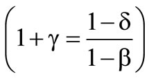 is illustrated in this figure. The value of the distribution at the optimal deductible above this border is
  and below

It can be concluded, that an insurer with  chooses the deductible in the amount of the greatest possible loss and consequently rejects the reinsurance.
In the case 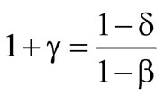 the value of the distribution at the optimal deductible fulfils

Hence the cedent decides in favour of the reinsurance. The border between accepting and rejecting the reinsurance depending on the profit mark-on of the reinsurer, is illustrated by the right figure of Chart 4.
It likewise can be recognized, that the purchase decision of the reinsurance moves in an area of higher risk aversion with increasing profit mark-on of the reinsurer. Consequently it is necessary that the higher the profit mark-on of the reinsurer is, the greater the risk aversion of the decision maker has to be, so that he purchases the reinsurance.
Concluding this, the following question remains: Which deductible, depending on the risk attitude with the b-d-preference functional, does the insurer choose in case of accepting the reinsurance? In this situation the value of the distribution at the optimal deductible decreases with an increase of risk aversion . That means, that the insurer wants to release more risk to the reinsurer. This is illustrated by Chart 5 for a given b.
Concerning both decision principles it can be concluded, that risk taking as well as risk neutral insurers reject the reinsurance. For risk aversion in contrast, two cases can be distinguished: On the one hand the case of lower risk aversion 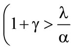 rather
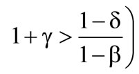 , where the reinsurance is rejected as well and on the other hand the case of higher risk aversion
 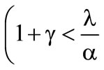 rather
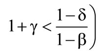 , where the insurer decides in favour of the reinsurance. That implies that only an insurer having enough risk aversion decides to take the reinsurance. In case that the reinsurance is accepted, the deductible decreases with the increase of risk aversion. It can be stated, that the higher the risk aversion is, the more risk is transferred to the reinsurer by the cedent. The interpretations of results are identical for both preference functionals. For this reason it is irrelevant, whether using the preference functional with the lower or with the upper expected value. It is possible to find for each a-l-combination of the first preference funktional a b-d-combination of the second preference funktional.
The analogy is .
.
6. Prospect
With the solutions of the optimal deductible it is possible to detect the risk preference of the insurer in case of knowing the loss distribution and the coverage limit. Furthermore the optimal deductible for a different assumed loss distribution can be calculated when knowing the risk preference of the insurer.
The introduced models only consider the maximization of the profit function in reference to the deductible. One possible prospect is the application of the hybrid decision model for the maximization of the profit function in reference to the cover or continuative the maximazation of a two dimensional model with deductible and cover.
Furthermore an investigation of the models could be made with the use of a fair premium and also the consistence to decision theories could be established.
7. References
[1] K. Gerathewohl, “Reinsurance principles and practice,” Vol. 1, Verlag Versicherungswirtschaft, Karlsruhe, 1980.
[2] E. Wollan, “Handbook of reinsurance law,” Aspen Publishers, New York, 2002.
[3] S. C. Bennett, “Dictionary of insurance, pearson education,” zug, 2004.
[4] E. Helland, C. R. Nysæter, “Solvency II: An Illustration, ” Forfatterne, Bergen, 2006.
[5] A. Schwepcke, D. Arndt, “Reinsurance: Principles and state of the art,” Verlag Versicherungswirtschaft, Karlsruhe, 2004.
[6] R. Phifer, “Reinsurance fundamentals: Treaty and facultative,” John Wiley, New York, 1996.
[7] M. Kaluszka, “Optimal reinsurance under mean-variance premium principles,” Insurance: Mathematics and Economics, Vol. 42, 2008.
[8] P. J. Montana, B. H. Charnov, “Management, Barron's educational series,” New York, 2000.
[9] V. Torra, Y. Narukawa, “Modeling Decisions for Artificial Intelligence,” Springer , 2009.
[10] G. Cachon and C. Terwiesch, “Matching supply with demand,” Mc Graw-Hill, New York, 2006.
[11] S. Chopra and P. Meindl, “Supply chain management,” 2. Edition, Prentice Hall, New Jersey, 2004.
[12] W. Jammernegg and P. Kischka, “A decision rule based on the conditional value at risk,” Jenaer Schriften zur Wirtschaftswissenschaft, Vol. 9, 2005.
[13] W. Jammernegg and P. Kischka, “Risk-averse and risk-taking newsvendors: A conditional expected value approach,” Review of Managerial Science, Vol. 1, 2007.
[14] K. Poser, M. Wagner, “Das Newsvendor Modell mit nicht-linearer Kostenfunktion und seine Anwendung bei nicht-proportionalen Rückversicherungsverträgen,” Jena Research Papers in Business and Economics, Vol. 15, 2007.
[15] P. Embrechts, R. Frey, and A. J. McNeil, “Quantitative risk management: Concepts,” Techniques and Tools, Princeton University Press, Oxford, 2005.
[16] M. Wagner, “Bestimmung von Deckungsgrenzen bei nicht-proportionalen Rueckversicherungsvertraegen,” German Journal of Risk and Insurance, Vol. 3, 2008.
Appendix
Proof of Theorem 1:
The following applies


The first derivation of the preference functional is generated and the following can be received

 .
.
At first the first differential of the expected profit and also of the conditional expected value has to be determined. For the profit function of the insurer can be assumed  For the expected profit can be obtained
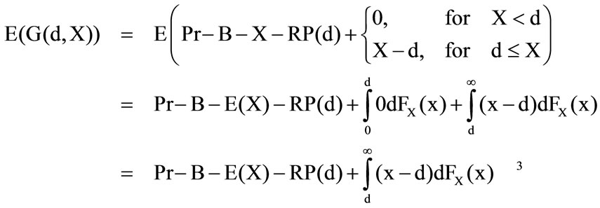

By the use of differentiation and the main theorem of the infinitesimal calculus for the expected profit follows

In the case  is for the conditional expected value essential, that

=
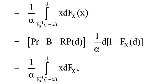
whereas  is the inverse function of the loss distribution. In general, the generalized lower inverse
 of the distribution function
  is required.
This has the following definition 
 , whereas
 . On the contrary, if one assumes a continuous and strictly increasing distribution function then the generalized lower inverse is equal to the inverse function
  of the loss distribution. In the following a continuous and strictly increasing distribution function should be assumed.
The first derivation of the conditional expected value is


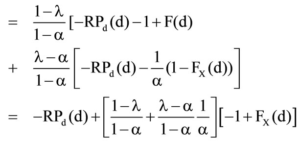
and so it is essential for the first derivation of the preference functional, that

 4
4
 5
5

Therefore the optimal solution  can be obtained. For the second derivation of the preference functional follows

It is necessary that  and
and  because the loss density is not negative. Hence
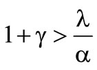
  is the maximum in the case of
 .
.
In the case  the conditional expected value is
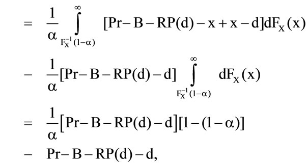

After differentiation it is necessary that .
.
Consequently for the first derivation of the preference functional can be obtained


 6
6

Therefore the optimal solution is
 .
.
Now the determination of the second derivation for the identification of the type of optimum can be made. It is necessary that
 .
.
As the loss density can not receive negative values, the second derivation of the preference functional is negative in case that . The following question arises: When does the optimum exist? At first
  is observed. This equation can be assumed, when the denominator of the solution is not negative. It is necessary, that

Therefore  is a maximum, for
 . The second step
is observed. It is necessary, that

and this is equivalent to , because

The result is, that the maximum exists, when the other maximum  does not exist.
NOTES
1These are the profits lying above the  -profit quantile.
2The proof of theorem Theorem 1 can be found in the appendix.
3It is necessary that


4It is necessary that 

5It is necessary that .
.
6It is necessary that .
.

