Journal of Electromagnetic Analysis and Applications
Vol. 2 No. 6 (2010) , Article ID: 2152 , 7 pages DOI:10.4236/jemaa.2010.26051
Voltage Generation by Rotating an Arbitrary-Shaped Metal Loop around Arbitrary Axis in the Presence of an Axial Current Distribution
![]()
National Technical University of Athens, School of Electrical and Computer Engineering, Division of Electromagnetics, Electrooptics and Electronic Materials, Athens, Greece.
Email: valagiannopoulos@gmail.com
Received March 1st, 2010; revised May 2nd, 2010; accepted May 7th, 2010.
Keywords: Electromagnetic Induction, Arbitrary-Shape Loop, Axial Current Excitation, Superposition Integral.
ABSTRACT
A thin metallic wire loop of arbitrary curvature is rotated with respect to an arbitrary axis of its plane. The device is excited by an electric dipole of infinite length and constant current. The resistance of the loop is computed rigorously as function of the position of the source. In this way, the induced voltage along the wire, under any kind of axial excitation, is given in the form of a superposition integral. The measured response is represented for various shapes of the coil, with respect to the time, the rotation angle and the position of the source. These diagrams lead to several technically applicable conclusions which are presented, discussed and justified.
1. Introduction
Electromagnetic (EM) induction is the production of voltage across a conductor situated in a changing magnetic field or a conductor moving through a stationary magnetic field. The physics that govern the inductive experiments have been mathematically examined in a number of old and elementary studies. The relationship between the various induction laws is summarized in [1] where Cohn advocates that the combined use of both motional and transformer induction assures the validity of the produced results. The Faraday’s disk, the typical DC generator, a cumulative magnet and other inductive structures are thoroughly investigated. Hvozdara also has contributed significantly in analyzing and solving rigorously some basic configurations where the EM induction phenomenon appears. For example in [2], the magnetotelluric field for a cylindrical inhomogeneity in a half space with anisotropic surface is evaluated, while in [3] is shown theoretically what effects are generated if one considers the rotation of a spherical Earth in an external inhomogeneous time-variable magnetic field. Moreover, a rudimentary study of induction in a rotating conductor surrounded by a rigid conductor of finite or infinite extent has been provided in [4]. The analysis is based on integral solutions of the field equations and leads to the conclusion that the induced magnetic fields depend on the relative symmetry of the rotator.
Many solving techniques have been utilized to convert the aforementioned theoretical analyses into practical applications in real-world configurations. For example in [5], a 3-D finite-element general method is presented to treat controlled-source induction problems in heterogeneous media. It can be used efficiently for EM modeling in mining, groundwater, and environmental geophysics in addition to fundamental studies of EM induction within a heterogeneous environment. Furthermore, many patents and inventions such as [6], exploit inductive phenomena to generate high-voltage power. In particular, the power capability of core-type transformers is increased by creating additional magnetomotive force in certain secondary coils without any subsequent power loss. Also in [7], a highly applicable technique is presented which describes finite-difference approximations to the equations of 2-D EM induction that permits discrete boundaries to have arbitrary geometrical relationships to the nodes.
Apart from the old standard textbooks and the newer technical reports, there are numerous recent, state-ofthe-art references examining devices and presenting techniques which exploit electromagnetic induction. In [8], a new electromagnetic induction detection mode for Capillary Electrophoresis (CE) and microfluidic chip CE has been presented. Its own optimal operating conditions are determined, and its application in CE and microfluidic chip CE of inorganic ions is described. A study [9] tests the validity of using electromagnetic induction (EMI) survey data, a new prediction-based sampling strategy and ordinary linear regression modeling to predict spatially variable feedlot surface manure accumulation. In addition, a flow injection system incorporating electromagnetic induction heating oxidation for on-line determination of chemical oxygen demand has been proposed [10]. The procedure utilizes induction heating instead of conventional reflux heating, with acidic potassium dichromate acting both as an oxidant and as a spectrometric reagent. Finally, a general-purpose analysis is contained in [11], where the law of induced electromotive force is applied to three significant cases: moving bar, Faraday’s and Corbino’s disc.
In this work, we assume a closed metallic wire of arbitrary shape which is mechanically rotated with respect to an arbitrary axis of its plane, in the presence of an elemental source of infinite length and constant current. The parametric equation of the wire curve is extracted through coordinate transformations and the magnetic flux through the loop is evaluated straightforwardly. To this end, we apply the Faraday’s law and an expression for the coil’s resistance is derived. This study examines the voltage induction to the most general case of a single wire loop (shape and rotation axis can be altered at will) which has not been treated rigorously yet. However, the basic novelty of the present analysis is that, due to the linearity of the participating operators, the calculus can be generalized to cover any case of axial excitation. We compute a kind of “Green’s function” ([12]) for the loop impedance, corresponding to a point source excitation. Therefore, the solution for more complex axial currents utilized in industry and technology is given through an integral of that resistance function multiplied by the current distribution of the source. A set of computer programs has been developed to evaluate the formulas, the induced voltage is represented as function of the time, the rotation angle and the position of the source for various loop shapes, while the produced graphs are presented and discussed.
2. Problem Statement
The Cartesian coordinate system  defined in Figure 1(a) will be used throughout the analysis. We suppose an infinite axial dipole into vacuum, parallel to
 ![]() axis, at the position
axis, at the position , flown by a constant current
  (in Amperes). A wire loop is located around the origin
  on the
  plane, and its shape is determined by the radial distance
  (polar function) where
 ![]() is the (unprimed) azimuthal angle of our consideration. This closed curve of a perfectly conducting material and infinitesimal thickness is rotated periodically around the arbitrary axis
is the (unprimed) azimuthal angle of our consideration. This closed curve of a perfectly conducting material and infinitesimal thickness is rotated periodically around the arbitrary axis  with circular frequency
![]() , as shown in Figure 1(b). Consequently, it makes sense just to examine the loop turned by the representative angle
, as shown in Figure 1(b). Consequently, it makes sense just to examine the loop turned by the representative angle  with
with

Figure 1. (a) The physical configuration of the device. An arbitrary-shaped loop is rotated periodically, in the presence of an infinite dipole, with respect to an axis parallel to the source; (b) The rotation is carried out with respect to an arbitrary axis
respect to the aforementioned axis. Initially , the curve lies entirely on the
  plane.
The purpose of this work is to obtain an expression for the electromotive force induced at the coil, being dependent on the time , the rotation axis
  and the shape of the loop
 . The generated voltage should certainly vary with the position of the primary source
 , and thus the derived formula could be used in studying structures with more complicatedly distributed excitation current.
3. Mathematical Formulation
Firstly, we should extract the parametric equation set of the rotated loop when  as appeared in Figure 1. The equations will be denoted by

 and the azimuthal angle
  will play the role of the parametric variable even when the object does not belong exclusively to
  plane. As the closed wire is rotated with respect to
 ![]() axis, the corresponding coordinate
axis, the corresponding coordinate  will be fixed, independent from the angle
  and equal to
 . The rest two equations are derived by projecting the other edge of length
 , which is posed at angle
 , upon the axes
 ![]() and
and . Accordingly, one obtains the following expressions:
 , (1)
, (1)
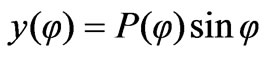 , (2)
, (2)
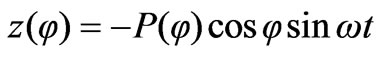 . (3)
. (3)
In order to find the parametric equation of the curve when , we use the primed coordinate system
  which is received through rotation of the unprimed one by angle
  with respect to axis
  (defined in Figure 1(b)). The polar equation of the loop is now given by
 , while the two azimuthal angles are connected obviously via the relation
 . Therefore, we take the Formulas (1)-(3) replacing
 ![]() by
by  and the unprimed variables
  by the primed ones
 . In this sense, the parametric set of the primed coordinates with respect to unprimed azimuthal angle
 ![]() (after trivial algebraic manipulations), is written as follows:
(after trivial algebraic manipulations), is written as follows:
 (4)
(4)
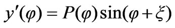 , (5)
, (5)
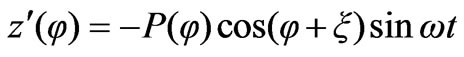 (6)
(6)
The parametric equations of the arbitrarily rotated wire loop expressed in the unprimed coordinate system are denoted by 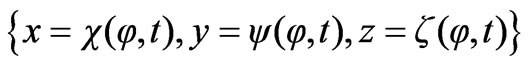 and are determined from the transformation relation below [13]:
 (7)
(7)
An extra time argument has been added to the dependencies of the parametric equations for better comprehension.
Once the boundary of the rotating wire is rigorously specified, the field quantities related to the induced voltage can be computed. The magnetic vector potential of a ![]() -polarized infinite dipole into vacuum at distance
-polarized infinite dipole into vacuum at distance  from its axis is given by [14]:
 , (8)
, (8)
where  is the reference distance,
  is the vacuum magnetic permeability and
 ![]() is the unitary vector of the
is the unitary vector of the ![]() axis. The transverse distance of the representative loop point with azimuthal angle
axis. The transverse distance of the representative loop point with azimuthal angle![]() , at an arbitrary time
, at an arbitrary time , from the axis
 , is found apparently equal to:
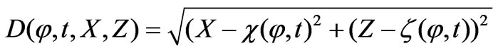 , (9)
, (9)
also shown in Figure 2. It is well-known [15] that the magnetic flux through a closed loop ![]() is defined from the line integral of the magnetic potential on the curve, that is
is defined from the line integral of the magnetic potential on the curve, that is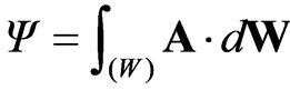 . In our case, this formula is particularized [16] to give:
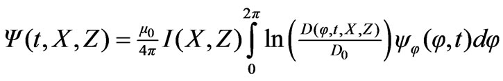 ,(10)
,(10)
where the subscript notation is used for the partial derivative of a function. It should be noted that the magnetic flux is independent from the reference distance . According to Faraday’s law, the induced electromotive force is given by the time derivative of magnetic flux
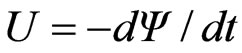 ; therefore, it is sensible to define the following auxiliary resistance function by excluding
 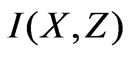 from (10):
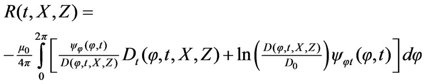 (11)
(11)

Figure 2. The transversal distance between the axis of the dipole and a representative point of the rotated loop projected on x-z plane
In this way, the generated voltage on the coil due to the self-rotation, in the presence of a dipole posed along the axis , is given by:
 (12)
(12)
In case the structure is excited by an axial surface current distributed according to the law 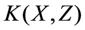 (measured in
 ), along the line
 , the induced electromotive force on the wire loop, is expressed in terms of the following line integral:
 (13)
(13)
Such an expansion is permissible because the operator  applied on
  to find
 , is linear. Similarly, if the excitation is a volume axial current
  (measured in
 ), across the area
 , the voltage is obtained through the double integral below:
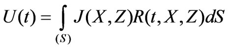 (14)
(14)
4. Indicative Results In this section, we examine the produced voltage by rotating loops of variable shape and the effect of their geometrical parameters on it. The described method is applied to two families (A, B) of wire boundaries possessing the following polar equations:
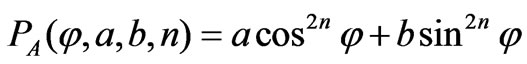 ,(15)
,(15)
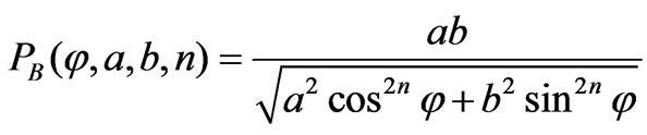 , (16)
The arguments  have length dimension and the argument
 ![]() is a positive integer number. For brevity, we chose to excite the structure exclusively through point sources avoiding surface or volume distributions described through (13), (14). The following graphs will exhibit the dependencies of the produced voltage
is a positive integer number. For brevity, we chose to excite the structure exclusively through point sources avoiding surface or volume distributions described through (13), (14). The following graphs will exhibit the dependencies of the produced voltage  and the corresponding RMS value:
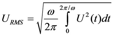 (17)
(17)
A single wire loop is not practically used for voltage generation as clusters of coils are utilized instead. We are more concerned for the qualitative description of the output quantity than measuring the exact magnitude (in Volts) of the produced voltage which is extremely small. Accordingly, the so-called “normalized voltage” is represented alternatively which is evaluated by replacing the magnetic permeability of the vacuum 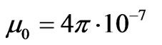
 in (11), by unity. Each figure below is divided into two subfigures, the first of which is a diagram depicting the variation of the investigated quantities for various shapes of the loop, while the second is a polar plot of the corresponding wire boundaries.
In Figure 3(a), we represent the time dependence of the developed normalized voltage for various shapes of loops corresponding to different ![]() parameters of the curve family A with constant
parameters of the curve family A with constant  and
and . The observation duration is a single period as from that point on the procedure and the results are repeated unchanged. Even though the shape of the wire is arbitrary, the waveforms exhibit typical sinusoidal behavior, a fact that can be attributed to the horizontal and vertical symmetry of the metallic loop boundary. Also, the amplitude of the oscillation gets greater, as the area of the closed wire increases. This is a natural conclusion because by keeping fixed the rotation frequency and the axis parallel to the dipole, larger loops lead to more significant magnetic flux variance and implicitly to more substantial output voltage. Therefore, the oscillation amplitude of the investigated quantity is decaying with increasing
 ![]() because the occupying area of the loop is greater for
because the occupying area of the loop is greater for  than for
  as shown in Figure 3(b).
In Figure 4(a), the variation of the RMS value of the induced voltage is depicted as function of the rotation angle  for three loop boundaries corresponding to different lengths
  of the curve family A with constant
  and
and . For
. For , the measured response is locally minimized when
  and maximized when
 . That is because the larger lobes of the curve extend close to the rotation axis in the first case and far from it in the second one as appeared in Figure 4(b). When
 , all the four lobes of the curve are of the same size, which means that the global maximum at
  reflects the rule according to which, better induction results are achieved when the current axis crosses normally the rotation axis of the coil. When
 , substantial voltage is produced for a rotation angle close to
 , where the response is poor in the case of
 . Needless to say that the graphs are symmetrical with respect to
 , due to the canonical shape of the loops.
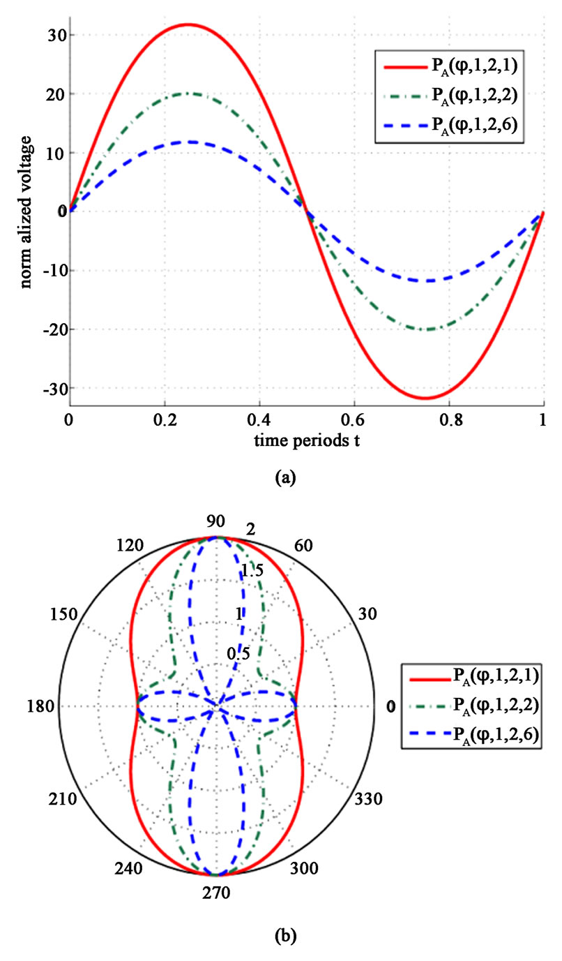
Figure 3. (a) The normalized voltage as function of time for various shapes of the loops. (b) The corresponding polar plots of the bounds. Plot parameters: ξ = 0o, X = -5 m, Z = 0 m, ω = 100π rad/sec, D0 = 1 m, I = 1 A, a = 1 m, b = 2 m
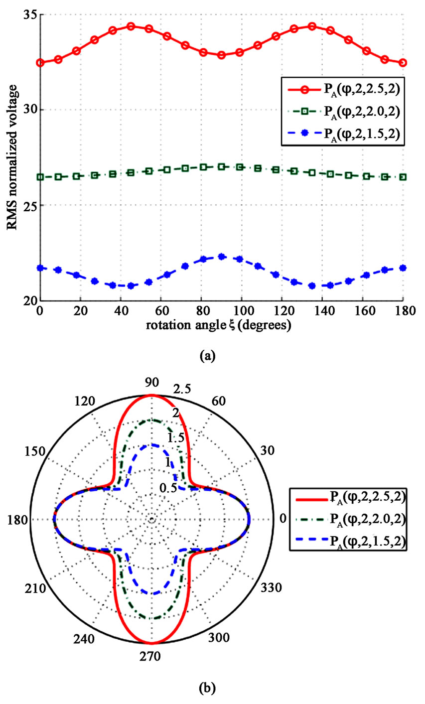
Figure 4. (a) The RMS voltage as function of the rotation angle for various shapes of the loops; (b) The corresponding polar plots of the bounds. Plot parameters: X =-5 m, Z = 0 m, ω = 100π rad/sec, D0 = 1 m, I = 1 A, a = 2 m, n = 2
In Figure 5(a), we represent the produced voltage as function of the horizontal position of the source  for three metallic loops with shapes taken from the curve family B for various parameters
 ![]() (
( and
and 
 ). With increasing
 , namely when the source gets closer to the loop, the induced voltage takes more substantial values. Such a conclusion is sensible because the effect of the field gets stronger and consequently, the change in magnetic flux through the closed loop (from a maximum point to zero) takes larger values. Mind that the increase is much more rapid for
  than in the other cases, a result which is attributed to the negligible distance between some points of this loop and the singular excitation axis when
 . Along this region, the recorded magnitude is much higher compared to other measurements of similar configurations such as

Figure 5. (a) The RMS voltage as function of the rotation angle for horizontal positions of the source. (b) The corresponding polar plots of the bounds. Plot parameters: ξ = 0ο, Z = 0 m, ω = 100π rad/sec, D0 = 1 m, I = 1 A, a = 1 m, b = 2 m
these of Figure 4(a). On the other hand, when the primary source gets farther from the rotated wire, its shape plays a rather insignificant role and the differences are mainly attributed to the size of the loop.
In Figure 6(a), the variation of the induced voltage is represented as function of the vertical position of the excitation  (the source is moving normally to the plane of the sheet) for various loops from curve family B corresponding to different lengths
  (with fixed
  and
and ). In all the three cases the response is maximized for
  which is a natural result because the loop is at the closest distance from the excitation axis. In addition, the curves are symmetrical with respect to
 , due to the fact that the loops are symmetric with respect to the rotation axis which is parallel to that of the source (
 ) as shown in Figure 6(b).
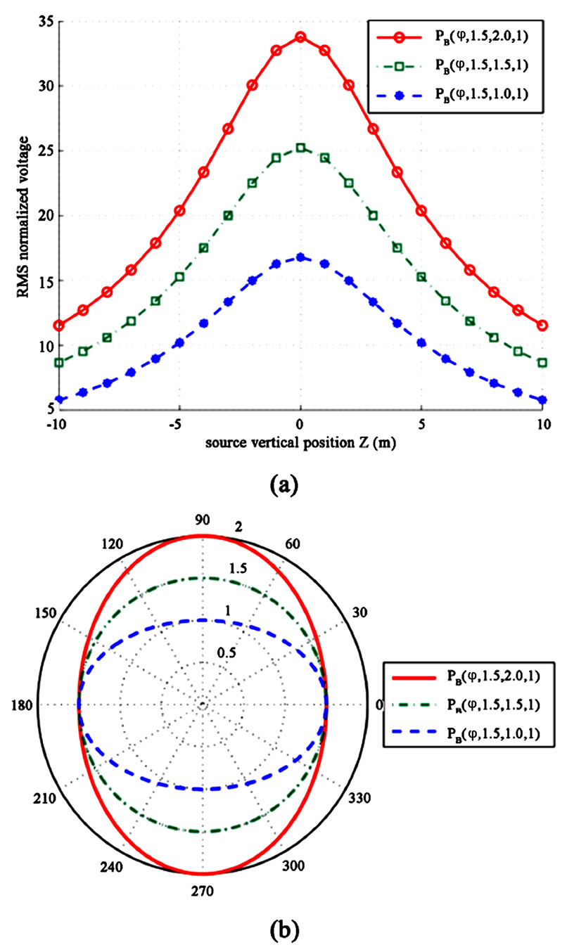
Figure 6. (a) The RMS voltage as function of the vertical position of the source for various shapes of the loops. (b) The corresponding polar plots of the bounds. Plot parameters: ξ = 0o, X = -5 m, ω = 100π rad/sec, D0 = 1 m, I = 1 A, a = 1.5 m, n = 1
One could point out that the positive effect of the coil’s size on the induced measured quantity is greater when the excitation field is stronger (larger differences between the three curves in the vicinity of ). It is also remarkable that the induced voltage is exponentially dependent on the distance between the thin closed wire and the source current, which is indicated not only by the decrease for large
  in Figure 6(a) but with the increase for large
  in Figure 5(a) as well.
5. Conclusions
The case of a metallic loop of arbitrary shape rotated with respect to an arbitrary axis in the presence of an infinite dipole is investigated. The induced voltage is evaluated rigorously via transformation relations and the derived formula can be easily generalized to treat any kind of axial excitation. The time dependence of the measured voltage is of sinusoidal form only if the shape of the loop combined with the rotation axis is symmetric. Additionally, the intuitive guess that the size of the loop, affects positively the inductive action is verified by the numerical results. The distance between the source and the loop is also found to reduce the measured voltage along the coil. As far as the rotation axis is concerned, the most substantial response has been recorded when it is normal to the axis of the dipole current, a result that can have technical applicability.
REFERENCES
- G. Cohn, “Electromagnetic Induction,” Electrical Engineering, Vol. 1, No. 1, May 1949, pp. 441-447.
- M. Hvodara and O. Praus, “Electromagnetic Induction in a Half-Space with a Cylindrical Inhomogeneity,” Studia Geophysica et Geodaetica, Vol. 16, No. 3, September 1972, pp. 240-261.
- M. Hvodara and O. Praus, “On Some Effects Connected with Electromagnetic Induction in a Rotating Earth,” Studia Geophysica et Geodaetica, Vol. 15, No. 2, June 1971, pp. 173-180.
- A. Herzenberg and F. Lowes, “Electromagnetic Induction in Rotating Conductors,” Philosophical Transactions of the Royal Society of London, Series A, Mathematical and Physical Sciences, Vol. 249, No. 970, May 1957, pp. 507- 584.
- E. Badea, M. Everett, G. Newman and O. Biro, “FiniteElement Analysis of Controlled-Source Electromagnetic Induction Using Coulomb-Gauged Potentials,” Geophysics, Vol. 66, No. 3, 2001, pp. 786-799.
- B. Skillicorn, “Electromagnetic Induction Apparatus for High-Voltage Power Generation,” United States Patent, No. 833436, October 1971.
- C. Aprea, J. Booker and J. Smith, “The Forward Problem of Electromagnetic Induction: Accurate Finite-Difference Approximations for Two-Dimensional Discrete Boundaries with Arbitrary Geometry,” Geophysical Journal International, Vol. 129, No. 1, 1996, pp. 29-40.
- Z. Chen, O. Lia, C. Liua and X. Yanga, “Electromagnetic Induction Detector with a Vertical Coil for Capillary Electrophoresis and Microfluidic Chip,” Sensors and Actuators B: Chemical, Vol. 141, No. 1, August 2009, pp. 130-133.
- B. Woodbury, S. Lesch, R. Eigenberg, D. Miller and M. Spiehs, “Electromagnetic Induction Sensor Data to Identify Areas of Manure Accumulation on a Feedlot Surface,” Soil Science Society of America Journal, Vol. 73, No. 6, November 2009, pp. 2068-2077.
- S. Han, W. Gan, X. Jiang, H. Zi and Q. Su, “Introduction of Electromagnetic Induction Heating Technique into onLine Chemical Oxygen Demand Determination,” International Journal of Environmental Analytical Chemistry, Vol. 90, No. 2, January 2010, pp. 137-147.
- G. Giuliani, “A General Law for Electromagnetic Induction,” Europhysics Letters, Vol. 81, No. 6, February 2008, pp. 1-6.
- C. Valagiannopoulos, “Arbitrary Currents on Circular Cylinder with Inhomogeneous Cladding and RCS Optimization,” Journal of Electromagnetic Waves and Applications, Vol. 21, No. 5, 2007, pp. 665-680.
- L. Hand and J. Finch, “Analytical Mechanics,” Cambridge University Press, Cambridge, 1998, pp. 260-261.
- M. Sadiku, “Elements of Electromagnetics Oxford Series in Electrical and Computer Engineering,” Oxford University Press, Oxford, pp. 284-290.
- E. Rothwell and M. Cloud, “Electromagnetics,” CRC Press, Florida, 2003.
- R. Wrede and M. Spiegel, “Advanced Calculus,” Schaumm’s Outline Series, 3rd Edition, BPB Publications, Delhi, pp. 229-232.