Journal of Electromagnetic Analysis and Applications
Vol. 2 No. 3 (2010) , Article ID: 1547 , 9 pages DOI:10.4236/jemaa.2010.23025
Exact Solutions of Equations for the Strongly-Conductive and Weakly-Conductive Magnetic Fluid Flow in a Horizontal Rectangular Channel
![]()
1School of mathematics and computational Science, Xiangtan University, Xiangtan, China; 2Department of Energy and Resources Engineering, College of Engineering, Peking University, Beijing, China; 3Faculty of Mechanical Engineering, Doshisha University, Kyoto, Japan.
Email: limingjun@xtu.edu.cn, alimingjun@163.com
Received April 1st, 2009; revised May 5th, 2009; accepted June 23rd, 2009.
Keywords: Magnetic Fluid, Variational Function, Conductivity Coefficient, Strongly-Conductive, Weakly-Conductive
ABSTRACT
This paper presents the results of exact solutions and numerical simulations of strongly-conductive and weakly-conductive magnetic fluid flows. The equations of magnetohydrodynamic (MHD) flows with different conductivity coefficients, which are independent of viscosity of fluids, are investigated in a horizontal rectangular channel under a magnetic field. The exact solutions are derived and the contours of exact solutions of the flow for magnetic induction modes are compared with numerical solutions. Also, two classes of variational functions on the flow and magnetic induction are discussed for different conductivity coefficients through the derived numerical solutions. The known results of the phenomenology of magnetohydrodynamics in a square channel with two perfectly conducting Hartmann-walls are just special cases of our results of magnetic fluid.
1. Introduction
The first classical study of electro-magnetic channel flow was carried out by Hartmann in the 1930s [1]. Hartmann’s well-known exact solution can be applied to very closely related problems in magneto-hydrodynamics (MHD) to appreciably simplify physical problems and give insights into new physical phenomena.
In magnetic fluids, the fluid dynamic phenolmena with magnetic induction create new difficulties for the solution of the problems under consideration. The classical Hartmann flow can be further generalized to include arbitrary electric energy extraction from or addition to the flow. In general, classical MHD flows are dealt with using the exact solution of the Couette flow which is presented when the magnetic Prandtl number is unity [1].
The exact solutions of appropriately simplified physical problems provide estimates for the approximate solutions of complex problems. In view of its physical importance, the flow in a channel with a considerable length, rectangular, two-dimensional, and unidirectional cross section, which is assumed steady, pressure-driven of an incompressible Newtonian liquid, is the simplest case to be considered. In such a flow, taking into account the symmetrical planes  and
and  and an exact solution is obtained by using the separation of variables. The solution indicates that, when the width-to-height ratio increases, the velocity contours become flatter away from the two vertical walls and that the flow away from the two walls is approximately one-dimensional (the dependence of
  on
on  is weak) [2].
If all walls are electrically insulating,  , Shercliff (1953) has investigated principle sketch of the phenomenology of Magnetohydrodynamics (MHD) channel flow of rectangular cross-section with Hartmann walls and side walls [3]. For perfectly conducting Hartmann walls,
  , Hunt (1965) gave velocity profile and current paths for different Hartmann number. They found that the current density is nearly constant in most of channel cross sections, the velocity distribution is flat, and the thickness of the side layers decreases with increasing intensity of
 , i.e. increasing Hartmann number [3]. Recently, Carletto, Bossis and Ceber defined the ratio magnetic energy of two aligned dipoles to the thermal energy
 , and their theory well predicts the experimental results in a constant unidirectional field [4]. Further results can be found in reference [5].
Other flow configurations in basic MHD may include Hele-Shaw cells. Wen et al. [6,7] were motivated to visualize the macroscopic magnetic flow fields in a square Hele-Shaw cell with shadow graphs for the first time, taking advantage of its small thickness and corresponding short optical depth. Examples of applications of MHD include the chemical distillatory processes, design of heat exchangers, channel type solar energy collectors and thermo-protection systems. Hence, the effects of combined magnetic forces due to the variations of magnetic fields on the laminar flow in horizontal rectangular channels are important in practice [8–10].
In the present study, we consider the characteristics of magnetic fluids in a horizontal rectangular channel under the magnetic fields and use the flow equations with a conductivity coefficient. The exact solutions of the strongly-conductive and weakly-conductive magnetic fluids are considered using the series expansion technique in order to obtain the relationship between the flow and magnetic induction. Also, a quadratic function on flow and magnetic induction is studied to verify the characteristic of flow field using the obtained solutions.
2. The Exact Solution of the Magnetic Fluid Equations
The configuration of the flow geometry is illustrated in Figure 1. The problem considered in this study is an incompressible steady flow in the positive x-direction with a magnetic field applied in the positive z-direction. The cross-section of the channel is given by the flow region 2 and 2
and 2 while the channel length is 2
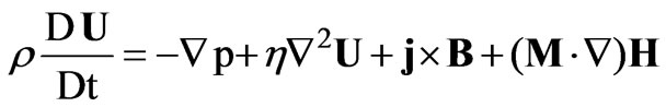
 . The system of basic magnetic fluid equations is given as follows [5]
 (1)
(1)
 (2)
(2)
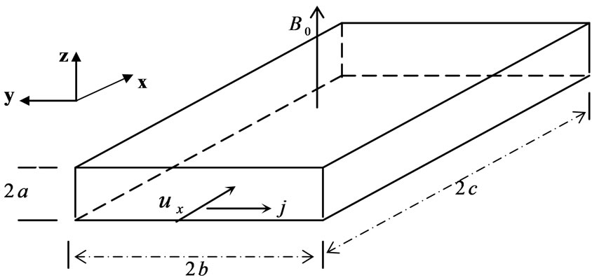
Figure 1. Illustration of flows in a rectangular channel
The Maxwell’s equations in their usual form
 ,
, ,
, (3)
(3)
with the relation equations and the Ohm’s law given as
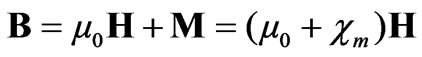 (4)
(4)
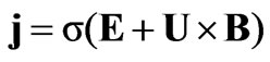 (5)
(5)
where  is the permeability of free space,
  is the magnetic susceptibility (H/m),
 is the conductivity,
  is the magnetic induction,
 is the magnetic field (A/m), and
  is the magnetization (A/m).
We choose the  axis such that the velocity vector of the fluid is
  and from the continuity Equation (1), we have
 . We also choose
  =
= , where
  is a constant representing magnetic induction.
Applying the Maxwell’s equation  and
and , we have
 . To simplify our presentations, the following assumptions are made for related variables:
 ,
, (6)
(6)
 ,
, (7)
(7)
 (8)
(8)
 ,
, (9)
(9)
And , Equation (3) is satisfied. As there is no excess charge in the fluid, then, by using (5),
  is obtained as follows
 (10)
(10)
 (11)
(11)
The magnetic fluid boundary conditions considered here are
 at
at ,
, 
 at
at ,
, 
We shall also assume that all quantities are independent of time , that is to say, the fluid we consider here is in a steady state.
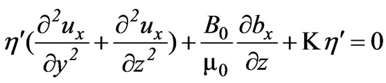
2.1 The Strongly-Conductive Fluid
The magnetic fluid is called strongly-conductive if the term  appears [8]. Under the condition of strongly conductive, the coefficient
  is much larger than the Kelvin force density
  so that
  is considered while
  is neglected. Using the steady-state assumption, i.e.,
  , Equation (2) can be written as follows
 (12)
(12)
 (13)
(13)
 (14)
(14)
where . Note that Sutton and Sherman [1] gave an incorrect result in their equation (10.85) which should be the above Equation (14).
For Hartmann flow, it is feasible to replace  by
by  for a simple model, then
  =
=
where .
.
The axial pressure gradient  is taken to be
  if the gravitational field is neglected, and
 , where
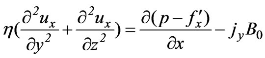
  is the viscosity of magnetic fluid. Combining Equations (12)–(14) yields
 (15)
(15)
 (16)
(16)
Let
 ,
, (17)
(17)
then Equations (15) and (16) are reduced to
 (18)
(18)
 (19)
(19)
where the Hartmann number  is defined as
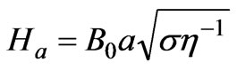 .
.
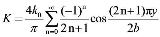
The solution for  is obtained by expressing
  over the range
  as a cosine Fourier series,
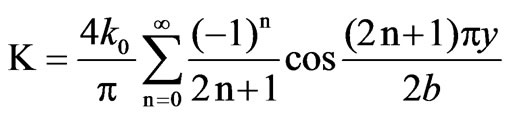 (20)
(20)
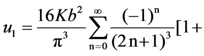
where  is a constant. The solution for
  is then written
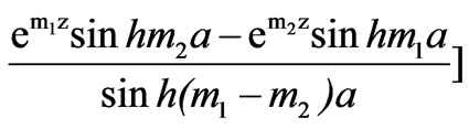
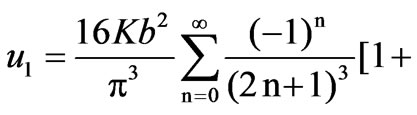 (21)
(21)
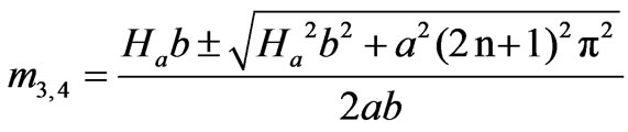
where  and
and  are given as
 (22)
(22)
It should be pointed out that the solution for  is just the same function as
  in which
  and
and  are displaced by
  and
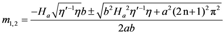
and , respectively, which are given by
 (23)
(23)
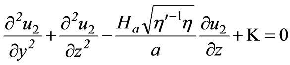
2.2 The Weakly-Conductive Fluid
If the fluid is weakly-conductive and the field  is not time-dependent, the term
  will disappear as shown in equations (104) [8]. Considering Equation (2) through (4) and making use of the assumptions mentioned above, the following relations are obtained,
 (24)
(24)
 (25)
(25)
 (26)
(26)
Replacing  with
with , we have
  =
= 
 as well as in Subsection 2.1. Then, as the axial pressure gradient
  is taken to be
 , where
 (27)
(27)
where  is a constant. Let
 ,
,  (28)
(28)
Thus, the solution of Equation (28) for  as in (17) is also obtained
 (29)
(29)
where  and
and  are as follows
 (30)
(30)
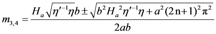
Note that the solution for  is the same function as
  in which
  and
and  are given as follows
 (31)
(31)
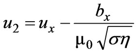
For a weak-conductive fluid, its solution is simply the solution of the conductive fluid with a conductive coefficient  (for
(for ). We find that
 which is obviously independent of the fluid viscosity.
2.3 Unidirectional Two Dimensional Flow without a Magnetic Field
Here we only consider a unidirectional two dimensional flow without a magnetic field, so that , Equations (18) and (19) are reduced to
 (32)
(32)
The boundary conditions are as follows
 at
at  (33)
(33)
 at
at  (34)
(34)
 at
at ,
, (35)
(35)
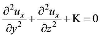
In order to obtain an exact solution of Equation (32), comparing with our above results, we have
 (36)
(36)
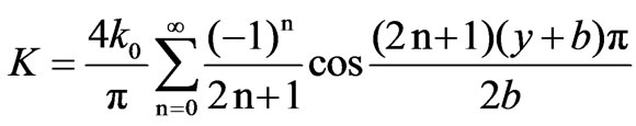
where  is a constant. The problem consisting Equation (32) and its conditions are solved similarly using the separation of variables, which has the solution as follows [9]
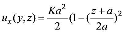
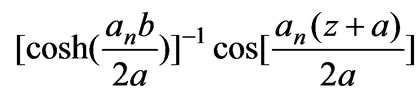 (37)
(37)
where
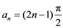 ,
, (38)
(38)
2.4 The Solutions, Flow Field and Discussions
In the present study, the flow fields and their associated functions are presented in the flow region with ,
, . Since
  ranges from 10 to 100 in most practical problems, the initial magnetic induction is taken to be
  (kg.s-2.A-1),
  (H/m),
  and the constant
 .
.
Figure 2 depicts the solutions for , 0.2 and 1.0, where
  is the conductivity coefficient. The velocity contours are displayed in Figure 2(a) for different values of the conductivity coefficient. It is shown that the velocity gradients become larger gradually near four vertical walls as the conductivity coefficient increases for different magnetic fluids. On the contrary, in the region of (0,0), the velocity gradients lower gradually as the conductivity coefficient increases. For the case of a constant Hartmann number, the magnetic fluid are shown in Figure 2(b) for different values of the conductivity coefficient, and as indicated, the strength of magnetic induction dampens horizontal away from the plane
  and the walls
  as the conductivity coefficient increases. On the contrary, near the walls
 , the magnetic induction becomes gradually low as the conductivity coefficient increases. For conductivity coefficient
 , the flow contours are similar to those in the reference[10] for the magnetic Rayleigh number
 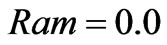 and the Rayleigh number
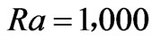 . Our analysis shows that the flow field changes with different conductivity coefficients.
Figure 3 shows the velocity fields for steady, unidirectional flows in a rectangular channel and  is a cosine Fourier series of
  and conductivity coefficient
 . The velocity contours are similar to those given by Papanastasiou et al. for the width-to-height ratio 1:1 [2].
In Figures 4(a) and 4(b), the development of the velocity profile in  and
and  directions are shown for various values of the conductivity coefficient
 . For the symmetry, we only consider two cases: (a)
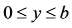 ,
, ; and (b)
 ,
, . Several interesting observations are readily made from the results. The cooperate process of
  and
and  is shown in the above analysis. In order to clearly show the self-governed process of
  and
and , the contours of the velocity versus coordinate
 , and the velocity versus coordinate
  are given. It is clear that the velocity gradients increase quickly near the boundary walls
  and
and  as
as  is increased. On the other hand, the exact solutions are multiple hyper-cosine functions of
 , and cosine functions of
 . Therefore, the velocity gra-
 (a)
(a) (b)
(b)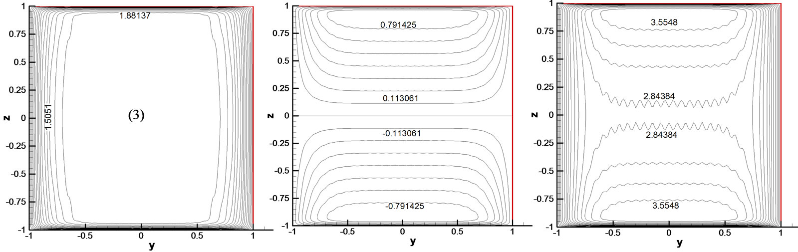 (c)
(c)
Figure 2. The distribution of flow field and magnetic induction. (a) Velocity contours ; (b) Magnetic induction distributions
 ; and (c) The velocity composition function
 . (1)
. (1) ,
, ; (2)
; (2) ,
, ; and (3)
 ,
, 
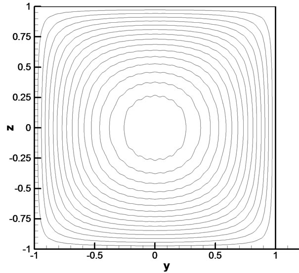
Figure 3. Velocity field with a cosine Fourier series  of
of  for conductive coefficient
dient is larger near the boundary walls than that near the boundary walls
  for a given
 .
.
For a given Hartmann number, comparing Figure 2 of this paper with Figures 3.2, 3.3 and 3.4 of Reference [3], current density distribution magnetic fluid and magnetohydrodynamics (MHD) are the same. Comparing Figure 2 of this paper with Figure 3.1 of Reference [3], the velocity profile of the phenomenology is also same for magnetic fluid and MHD. Of course, magnetic fluid and MHD have different equations and formulations of the Hartmann number. For magnetic fluid, the constitutive equation is , the Hartmann number
 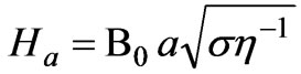 and conductivity coefficient
  are introduced in our work. The flow and magnetic induction
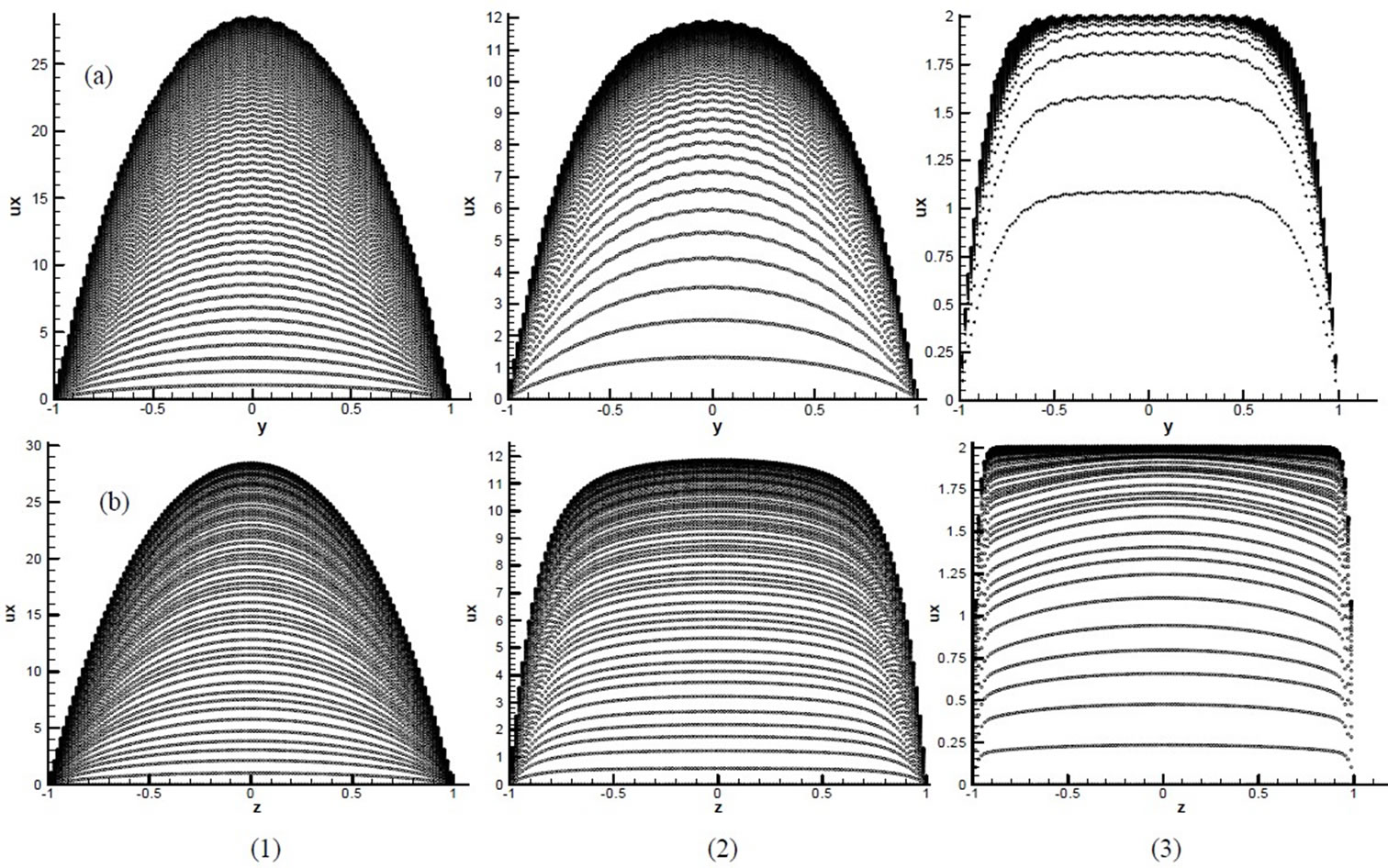
Figure 4. The development of the velocity profile (a) The  vs y-axis; (b)
  vs z-axis. (1)
 ,
, ; (2)
; (2) ,
, ; (3)
; (3) ,
, 
change with different . Differently, in MHD, Shercliff and Hunt considered the induction equation
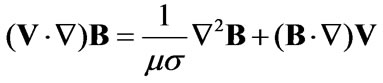 and used only the linear constitutive equation
  with Hartmann number
 . They gave velocity profile and current paths for different Hartmann number.
3. Two Class of Variational Functions on the Flow and Magnetic Induction
For many years the variation techniques have been effectively applied to problems in the theory of elasticity. However, they are rarely used in fluid dynamic problems. The great utility in elasticity problems are due to the fact that they can be conveniently applied to linear problems. This, of course, explains why they are not frequently used in fluid dynamics since most such problems are nonlinear [10,11].
For the conductive fluid problems of the type being considered here, we recall the governing Equations (15) and (16) which are linear for  and
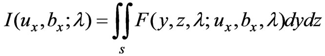
and  and the variation technique may be tried. Firstly, consider the following integral [12]
 (39)
(39)
where  is some given function of
 ,
, ,
, . Clearly, the value of the integral depends on the choice of the functions
 ,
,  and
and . Now, let us pose the following problem: to obtain functions
 ,
,  and
and  to minimize the value of
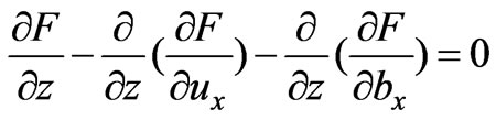
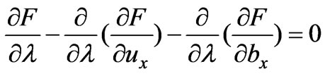
 . As is well known from variational calculus, the necessary conditions that
 ,
,  and
and  for minimized
  are the Euler equations:
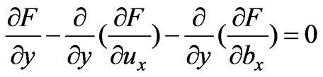 (40)
(40)
 (41)
(41)
 (42)
(42)
3.1 Decomposition and Composition Functions on the Flow and Magnetic Induction
Simply, let the parameters be fixed at , then
 . According to
  and
and  in the Equation (17), we only considered the function of
 ,
,  and
and  in order to minimize the special function as follows
 (43)
(43)
where  and
and  are considered as the function of
 ,
,  and
and ,
,  ,
,  , and
, and .
.
Let ,
, 
 , then
 . The expressions of
  and
and  are called the velocity decompositions of the magnetic induction
  and the flow field
  with a variable coefficient
  of the flow and the magnetic induction, where
 . From Figure 5, it is easy to show that
 ,
,  , and
, and 
 as
as , where
  is the velocity composition of the flow field and the magnetic induction.
It is also easy to know that  has the same variation characteristic as the following function
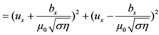
 (44)
(44)
The differential of  on
on  is given by
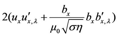
 (45)
(45)
It is obvious that  is a nonlinear function of
 , and is very complex to study the variation characteristics of
  by using the method of mathematical analysis.
With Equation (45), the variation characteristics of the function  is determined by flow and magnetic induction as a function of
 .
.
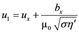
3.2 A Total Energy Variational Function on the Flow and Magnetic Induction
Based on the above analysis of Equation (17), let
 ,
, 
 with
with
 , we call
  the velocity of magnetic fluid flow, which is equivalence to the velocity of magnetic fluid flow evoked by magnetic force. A total energy function is defined by
 =
= +
+  (46)
(46)
where  is the kinetic energy,
  is the magnetic energy.
By the calculus of variations, we have
 =
= +
+  (47)
(47)
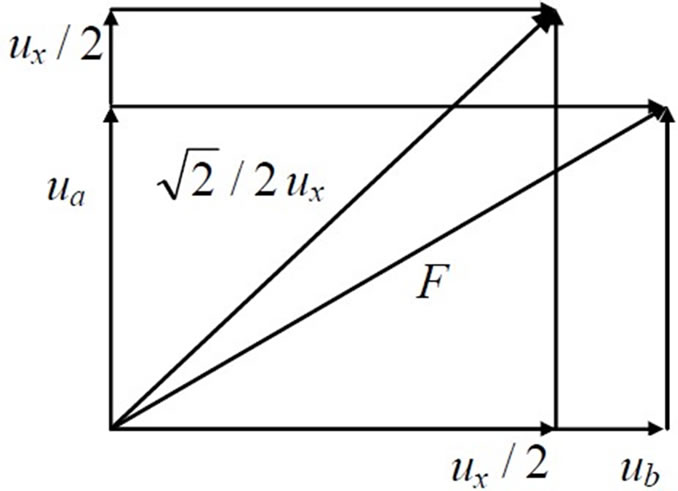
Figure 5. The sketch map of the composition function  of flow and magnetic induction
As  and
and  are nonlinear functions of
 , it is very complex to study the variational characteristics of
  by using the method of mathematical analysis.
3.3 Numerical Calculations and Discussions
As seen in Figures 2(a) and 2(c), in a region of (0,0), the contour of the function  is more similar to that of the flow for
 . Furthermore, the gradient of flow which is larger than that of magnetic induction, the distribution value of
  is largely affected depending on the flow. On the contrary, for
 , the gradient of magnetic induction is larger than that of flow as
  is largely affected depending upon the gradient of the magnetic induction.
It is observed that the difference of flow and magnetic induction are almost the same for  in a region of (0,0), where the distribution of the function
  is determined by the gradients of both the magnetic induction and the flow in this region. Furthermore, near
  and
and  for any
 , the difference of flow is acute singularly and the function
  is also changed singularly. It is noted that
  has only one limit point for
 , and F has two limit points for
 .
.
As seen in Figure 6, the gradient of the total energy is decided by the kinetic energy in the region (0,0) for different values of , and near
 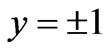 and
and  for
for . That is to say, the gradient of the magnetic energy is very large near
  for
for , and its value is very small which does not affect the gradient of the total energy. Then, the gradient of the total energy will be affected by the magnetic energy near
  for
for  and it will be affected by the magnetic energy near
  and
and  for
for .
.
4. Concluding Remarks
1) For magnetic fluid of this work and Magnetohydrodynamics (MHD) of Reference [3], the constitutive equa-
 (a)
(a)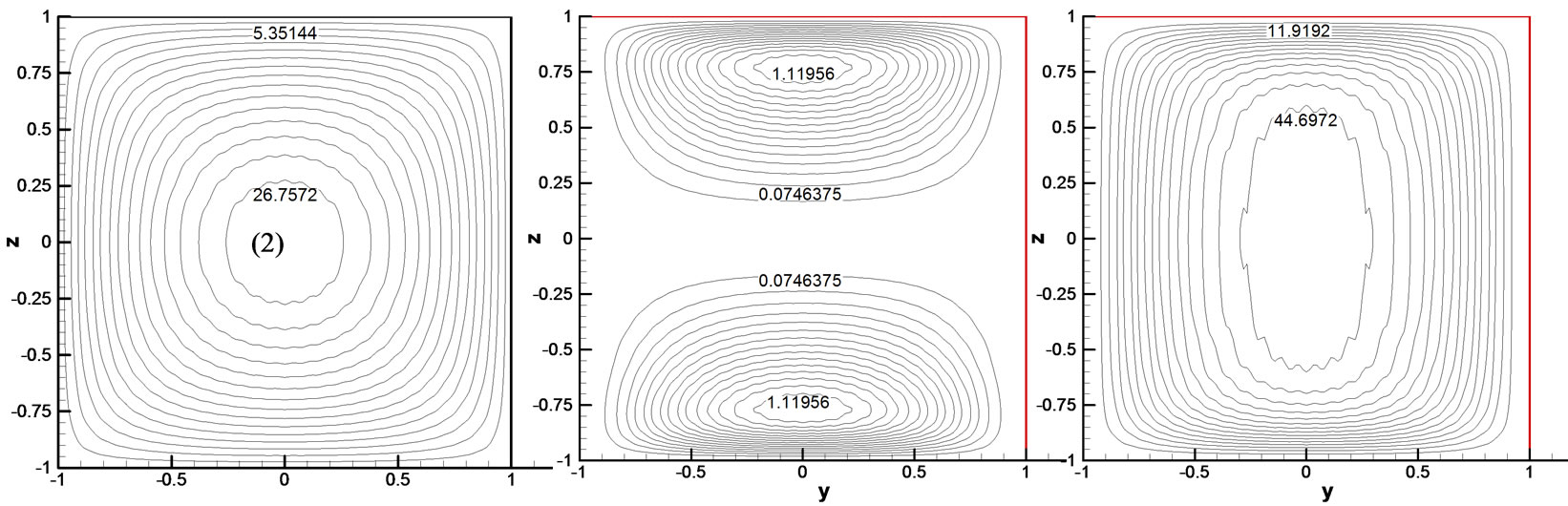 (b)
(b)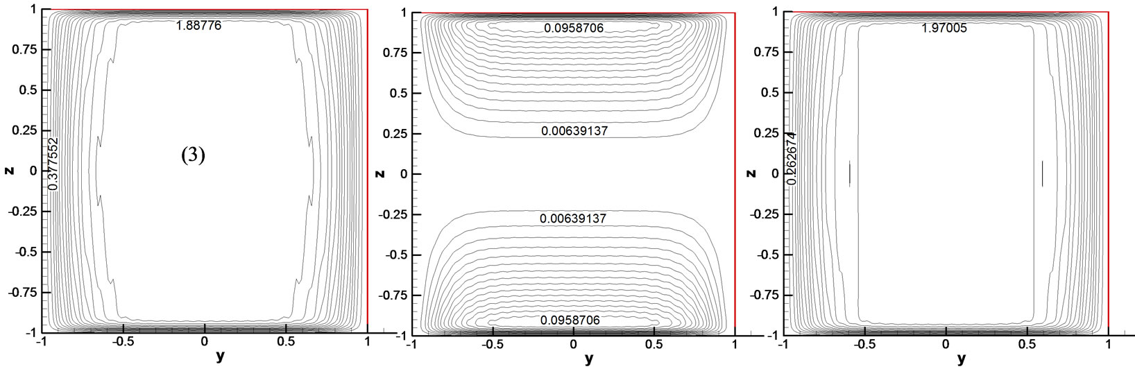 (c)
(c)
Figure 6. Illustration of energy function (a) The kinetic energy ; (b) The magnetic energy
 ; and (c) The total energy
 . (1)
. (1) ,
, ; (2)
; (2) ,
, ; (3)
; (3) ,
, 
tions are different, the Hartmann numbers are also different. For magnetic fluid, conductivity coefficient  is an important coefficient to analyze the flow and the current. For MHD, Hartmann number
  is the controlling coefficient, Shercliff and Hunt studied velocity profile and current paths for different Hartmann number [3–5].
2) For conductivity coefficient , the velocity contours for steady unidirectional flow is shown in a rectangular channel with
  a cosine Fourier series function of
 . Our result is in agreement with published findings.
3) A velocity decomposition and composition function , and a total energy variational function
 , on the flow and magnetic induction are considered. The variational characteristics of
  are analyzed only using the characteristics of the resultant flow field and the magnetic induction, and the number of its limit points changes as
  changes. It is shown in numerical simulations that the gradient of total energy
  is affected by the kinetic energy and the magnetic energy as
  changes.
4) Theoretically, the strongly-conductive and weaklyconductive magnetic fluid flows are studied on different conductivity coefficients which are independent of fluid viscosity in a horizontal rectangular channel.
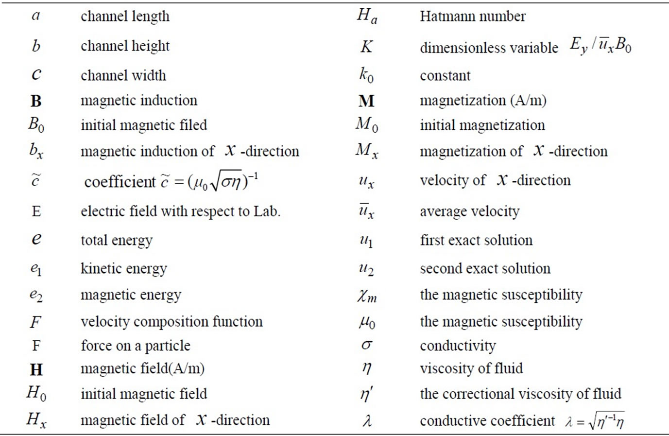
Table 1. Nomenclature
5. Acknowledgments
This work was supported in part by a grant to the research Centre for Advanced Science and Technology at Doshisha University from the Ministry of Education, Japan; the National Natural Science of China (10771178, 50675185, 10676031); the Research Fund for the Doctoral Program of Higher Education (20070530003), Program for New Century Excellent Talents in University (NCET 06-0708)and the Scientific Research Foundation for the Returned Overseas Chinese Scholars of State Education Ministry of China. The authors thank readers for giving references [3–5] and suggestions on comparison with analytical solutions.
REFERENCES
- G. W. Sutton and A. Sherman, “Engineering Magnetohydrodynamics,” McGraw-Hill Book Company, New York, 1965.
- T. C. Papanastasiou, G. C. Georgiou, and A. N. Alexandrou, “Viscous fluid flow,” CRC Press LLC, New York, 2000.
- U. Mueller and L. Buehler, “Magnetofluiddynamics in channel and containers,” Springer-Verlag, Berlin, 2001.
- P. Carletto, G. Bossis, and A. Cebers, “Structures in a magnetic suspension subjected to unidirectional and rotating field,” International Journal of Modern Physics B, Vol. 16, No. 17–18, pp. 2279–2285, 2002.
- E. Blums, A. Cebers, and M. M. Maiorov, “Magnetic fluids,” Walter de G Gruyter, Berlin, 1997.
- C.-Y. Wen and W.-P. Su, “Natural convection of magnetic fluid in a rectangular Hele-Shaw,” Journal of Magnetism and Magnetic Materials, Vol. 289, pp. 299– 302, March 2005.
- C.-Y. Wen, C.-Y. Chen, and S.-F. Yang, “Flow visualization of natural convection of magnetic fluid in a rectangular Hele-Shaw cell,” Journal of Magnetism and Magnetic Materials, Vol. 252, pp. 206–208, November 2002.
- R. E. Rosensweig, “Ferrofluids: Magnetically controllable fluids and its applications,” In: S. Odenbach, Ed., Basic Equations for Magnetic Fluids with Internal Rotations, Springer-Verlag, New York, p. 61, 2002.
- T. H. Kuehn and R. J. Goldstein, “An experimental study of natural convection heat transfer in concentric and eccentric horizontal cylindrical annuli,” ASME Journal of Heat Transfer, Vol. 100, pp. 635–640, 1978.
- H. Yamaguchi, Z. Zhang, S. Shuchi, and K. Shimad, “Heat transfer characteristics of magnetic fluid in a partitioned rectangular box,” Journal of Magnetism and Magnetic Materials, Vol. 252, pp. 203–205, November 2002.
- G. B. Arfken and H. J. Weber, “Mathematical methods for physicists,” 6th Edition, Elsevier Academic Press, New York, p. 1037, 2005.
- H. Yamaguchi, “Engineering fluid mechanics,” SpringerVerlag, New York, 2008.