Int'l J. of Communications, Network and System Sciences
Vol. 5 No. 6 (2012) , Article ID: 19662 , 18 pages DOI:10.4236/ijcns.2012.56047
Dynamic Clustering with Relay Nodes (DCRN): A Clustering Technique to Maximize Stability in Wireless Sensor Networks with Relay Nodes
School of ECE, Purdue University, West Lafayette, USA
Email: {bmalima, sajjad, vr}@purdue.edu
Received January 25, 2012; revised March 4, 2012; accepted April 24, 2012
Keywords: Network Stability Period; Clustering; Energy Consumption Rate; Relay Node
ABSTRACT
With the growing popularity of wireless sensor networks, network stability has become a key area of current research. Different applications of wireless sensor networks demand stable sensing, coverage, and connectivity throughout their operational periods. In some cases, the death of just a single sensor node might disrupt the stability of the entire network. Therefore, a number of techniques have been proposed to improve the network stability. Clustering is one of the most commonly used techniques in this regard. Most clustering techniques assume the presence of high power sensor nodes called relay nodes and implicitly assume that these relay nodes serve as cluster heads in the network. This assumption may lead to faulty network behavior when any of the relay nodes becomes unavailable to its followers. Moreover, relay node based clustering techniques do not address the heterogeneity of sensor nodes in terms of their residual energies, which frequently occur during the operation of a network. To address these two issues, we present a novel clustering technique, Dynamic Clustering with Relay Nodes (DCRN), by considering the heterogeneity in residual battery capacity and by removing the assumption that relay nodes always serve as cluster-heads. We use an essence of the underlying mechanism of LEACH (Low-Energy Adaptive Clustering Hierarchy), which is one of the most popular clustering solutions for wireless sensor networks. In our work, we present four heuristics to increase network stability periods in terms of the time elapsed before the death of the first node in the network. Based on the proposed heuristics, we devise an algorithm for DCRN and formulate a mathematical model for its long-term rate of energy consumption. Further, we calculate the optimal percentage of relay nodes from our mathematical model. Finally, we verify the efficiency of DCRN and correctness of the mathematical model by exhaustive simulation results. Our simulation results reveal that DCRN enhances the network stability period by a significant margin in comparison to LEACH and its best-known variant.
1. Introduction
With the emergence of highly dense fabrication technology and low production costs, Wireless Sensor Networks (WSNs) prove to be useful in a myriad of diversified applications. In a typical WSN application, sensor nodes are scattered in a region from where they collect data to achieve certain goals. Data collection may be continuous, periodic, or event based. Regardless of the data collection technique used, WSNs must operate in a stable manner. This stability is especially important in applications such as security monitoring and motion tracking. The death of just one sensor node may disrupt coverage or connectivity, and thus may reduce network stability in such applications. Therefore, it is important to ensure that all the deployed sensor nodes in WSNs be active during the operational lifetime to ensure uninterrupted service. However, sensor nodes are generally equipped with batteries that have a limited capacity. Therefore, each sensor node must efficiently use its available energy in order to improve the lifetime of the WSN. Different techniques have been proposed to ensure efficient usage of the available energy in a sensor node. Clustering is one of the most well known techniques used to ensure the efficient usage of the battery reserve of the sensor nodes.
Clustering techniques group deployed sensor nodes into clusters. One sensor node in a cluster is solely responsible for communicating with the base station. This sensor node is called the cluster head, and the remaining sensor nodes in the cluster are called followers. Here, the followers collect data and send the collected data to their corresponding cluster heads. Afterwards, the cluster heads aggregate their own collected data with the data received from their followers and send the aggregated data to a base station or sink to accomplish a specific goal. Generally, cluster heads are physically closer to their follower nodes compared to the sink/base-station. Therefore, it takes less energy to transmit data to the cluster head instead of the sink, which allows the sensor nodes to conserve energy and live longer.
There are different clustering techniques in use for wireless ad-hoc networks. However, those techniques cannot be directly used in WSNs because of the fact that WSNs have stricter energy constraints than ad-hoc networks. Therefore, several clustering techniques are proposed in the literature to specifically focus on the constraints of WSNs. We can categorize these clustering techniques in two groups—static and dynamic. Dynamic clustering techniques are more useful for WSNs because they can exploit the dynamic variation in residual energies of the sensor nodes, and thus can maximize network lifetime to a great extent. Different dynamic clustering techniques consider the lifetime of sensor networks in different ways in their optimization processes.
In some early research, network lifetime of a WSN is considered as the time required by the last sensor node to die. Some other research considers the lifetime of a WSN in a different way—the time required by half of the sensor nodes to die. However, network lifetime is frequently defined as n-of-n lifetime [1] that implies the time required by the first sensor node to die. We refer to this duration as the stability period of a WSN. There is an impact of efficient usage of available energy in a sensor node on the stability period of a WSN. Deployment of high-energy sensor nodes called relay nodes can greatly increase the efficiency of usage of available sensor energy. In this paper, we propose a novel technique called Dynamic Clustering with Relay Nodes (DCRN), which ensures efficient usage of the available energy throughout the network by taking advantage of both the clustering and deployment of relay nodes. To the best of our knowledge, all research studies that use relay nodes mainly attempt to optimize their placements by considering them as cluster heads. However, this approach suffers from the following limitations:
· Failure of relay nodes causes faulty behavior in the network, and thus the approach makes the network less fault tolerant.
· After a significant amount of service time, the residual energies of relay nodes may become comparable to other live nodes in the network. In this case, the fixed assignment of cluster headships to relay nodes forces them to die even quicker than other live nodes, resulting in faulty behavior and lower network stability.
Therefore, we consider all sensor nodes as candidates for attaining cluster headships. This consideration enables us to avoid the limitations raised from the assumption of previous work.
We use LEACH [2], a simple but popular dynamic clustering technique used in WSNs, as the underlying approach of DCRN. LEACH effectively rotates cluster headship among the sensor nodes of a network based only on some locally available information. However, LEACH only considers homogeneous sensor nodes and does not consider the variation in residual energies of the sensor nodes when it selects the cluster heads. There are some already proposed modifications of LEACH to incorporate the variation. However, none of the modifications considers the deployment of relay nodes. Therefore, we consider the deployment of relay nodes as well as the variation in DCRN. We incorporate the balanced use of residual energy all over the network with the help of four heuristics in DCRN. Besides, we formulate a mathematical model for DCRN. Simulation results show that DCRN achieves a significant improvement in network stability over LEACH and its best variant.
Based on our work, we make the following set of contributions in this paper:
· We propose a novel distributed and dynamic algorithm to cluster a wireless sensor network with relay nodes to improve its network stability in terms of death of the first sensor node. The algorithm is based on four carefully devised heuristics.
· We adopt a mathematical model for our algorithm. The model can effectively find out the optimal percentage of relay nodes. We verify the optimality of our proposed model by comparing its suggested optimal percentage of relay nodes to that suggested by the model of LEACH.
· We demonstrate effectiveness of our proposed algorithm using extensive simulations to compare it with LEACH and the best variant of LEACH. Our simulation results show that our proposed algorithm can achieve up to 188% and 112% improvements in time before the death of the first node in comparison to LEACH and the best variant. Besides, our algorithm also improves the time before the death of half of the nodes by 23% and 15% in comparison to LEACH and the best variant.
We organize the rest of this paper as follows: We point out some related work in the following section. Then, we briefly describe the underlying approach of our technique along with its variants in Section 3. We present our proposed clustering technique with four heuristics and a complete mathematical model after that section. In Section 5, we evaluate the stability period of DCRN by simulation results. In the last two sections, we conclude the paper by discussing our future directions.
2. Related Work
Several techniques have already been proposed to improve network lifetime in WSN. Clustering is one of the widely accepted techniques among them. Clustering is also used in wireless ad-hoc networks and mobile ad-hoc networks. Several clustering techniques have already been introduced for partitioning nodes in these areas. Some of the early clustering techniques are—Hierarchical Clustering [3], Distributed Clustering Algorithm (DCA) [4], Spanning Tree (or BFS Tree) based Clustering [5], Clustering with On-Demand Routing [6], Clusering based on Degree or Lowest Identifier Heuristics [7], Distributed and Energy-Efficient Clustering [8], and Adaptive Power-Aware Clustering [9]. Some of the recently developed clustering techniques are PEGASIS (PowerEfficient Gathering in Sensor Information Systems) [10], Energy Efficient Clustering Routing [11], PEACH (Power Efficient And Adaptive Clustering Hierarchy) [12], Optimal Energy Aware Clustering [13], ACE (Algorithm for Cluster Establishment) [14], HEED (Hybrid EnergyEfficient Distributed Clustering) [15], PADCP (Power Aware Dynamic Clustering Protocol) [16], LEACH (LowEnergy Adaptive Clustering Hierarchy) [2], SEP (Stable Election Protocol) [17], and LEACH with Deterministic Cluster Head Selection [18].
PEGASIS [10] introduces a near optimal chain-based protocol. Here, each node communicates only with a close neighbor and takes turns transmitting to the base station, thus reducing the amount of energy spent per round. It assumes that all nodes have global knowledge of the network and employ the greedy algorithm. It maps the problem of having close neighbors for all nodes to the traveling salesman problem. PEGASIS is a greedy chain protocol that is near optimal for a data-gathering problem in sensor networks. A greedy approach considers the physical distance only, ignoring the capability of a prospective node on the chain. Hence, a node with a shorter distance but less residual energy may be chosen in the chain and may die quickly.
In [11], a cluster-based routing algorithm is proposed that combines hierarchical routing and geographical routing. The process of packet forwarding from the source nodes in the target region to the base station consists of two phases: inter-cluster routing and intra-cluster routing. For inter-cluster routing, a greedy algorithm is adopted to forward packets from the cluster heads of the target regions to the base station. For intra-cluster routing, a simple flooding is used to flood the packet inside the cluster when the number of intra-cluster nodes is less than a predetermined threshold. Otherwise, the recursive geographic forwarding approach is used to disseminate the packet inside the target cluster, i.e., the cluster head divides the target cluster into some sub-regions, creates the same number of new copies of the query packet, and then disseminates these copies to a central node in each sub region. Similar to [10], it uses a greedy algorithm based only on the distance, but not on the capability or the residual energy. Although it deals with the optimal forwarding approach, the criteria to choose the cluster heads optimally is not clearly explained.
PEACH [12] is a cluster formation technique based on overheard information from the sensor nodes. According to this approach, if a cluster head node becomes an intermediate node of a transmission, it first sets the sink node as its next hop. Then it sets a timer to receive and aggregate multiple packets from the nodes in the cluster set for a pre-specified time. It checks whether the distance between this node and the original destination node is shorter than that between this node and the alreadyselected next hop node. If the distance is shorter, this node joins to the cluster of the original destination node and the next hop of this node is changed to the original destination node. PEACH is an adaptive clustering approach for multi-hop inter-cluster communication. However, it suffers from almost the same limitations of PEGASIS due to the choice of physical propinquity.
Optimal energy aware clustering [13] solves the balanced k-clustering problem optimally, where k signifies the number of master nodes that can be in the network. The algorithm is based on the minimum weight matching. It attempts to optimize the sum of spatial distances between the member sensor nodes and the master nodes throughout the whole network. Further, it also attempts to effectively distribute the network load to all the masters, and thus to reduces the communication overhead and the energy dissipation. However, this research does not consider the residual energy level while choosing a node as the master. Hence, the choice of the master or cluster head is far away from the optimal energy efficient distribution of the cluster heads.
ACE [14] is a distributed clustering algorithm that establishes clusters into two phases—spawning and migration. There are several iterations in each phase and the gap between two successive iterations follows uniform distribution. During the spawning phase, new clusters are formed in a self-elective manner. When a node decides to become a cluster head, it will broadcast a message to its neighbors to become its followers. During the migration phase, existing clusters are maintained and rearranged, if required. Migration of an existing cluster is controlled by the cluster head. Each cluster head will periodically poll all of its followers to determine which could be the best candidate to elect as a new leader for the cluster. The current cluster head will promote the best candidate as the new cluster head and abdicate itself from its position. ACE results in uniform cluster formation with a packing efficiency close to hexagonal close-packing. HoweverACE does not consider the residual energy of the nodes while selecting cluster heads. Hence, the clustering is far away from the optimal energy efficiency.
HEED [15] introduces a distributed algorithm considering the residual energy of sensor nodes. It results in several clusters in a WSN by uniformly distributing the cluster heads over the network. It periodically selects cluster heads according to a hybrid parameter, which consists of a primary parameter, the residual energy of a node, and a secondary parameter, such as propinquity of a node to its neighbors or node degree. HEED converges in O(1) iterations using low messaging overhead and achieves fairly uniform cluster head distribution across the network. However, it chooses the initial percentage of cluster heads randomly. This random choice remains as a severe limitation of this algorithm.
PADCP [16] uses several adaptive schemes like dynamic cluster range, dynamic transmission power, and cluster head re-election to form clusters. In this approach, the sensor nodes are assumed to have the same transmission capability and the ability to adjust transmission power in five levels. PADCP has four major phases— neighbor information collection, cluster head election using a cost function, cluster formation using HEED, and cluster head re-election in the case of residual energy lower than a pre-defined threshold value. The mobility of the sensor nodes is considered in cluster formation. However, it suffers from the same randomly chosen initial probability limitations of HEED as it completely fol lows the HEED algorithm for cluster formation in its third phase. Moreover, there is no suggestion about the optimal weights of the cost function used in cluster head selection and the threshold used in cluster head re-election.
LEACH [2] introduces a simple mechanism for localized coordination and control for cluster set-up and operation. It also introduces the randomized rotation of the cluster heads and the corresponding clusters. However, it does not consider the variation of the initial energy nor the residual energy of sensors during cluster head selection. SEP [17], a LEACH variant, modifies the equation of the threshold. However, it considers only two types of nodes, normal and advanced, instead of the many types that can be encountered in the wireless sensor network after a significant amount of time of operation. Besides, Deterministic Cluster Head Selection (DCHS) [18], another variant of LEACH, also modifies the threshold to accommodate the heterogeneity of residual energy based on some heuristics. In addition, LEACH-C, proposed by the same authors of LEACH in [19], is a centralized technique which selects the cluster heads based on their positions. It considers a uniform distribution of the cluster heads based on their positions and the average residual energy in the network. However, it does not consider the relative residual energy in each sensor node. Finally, Adaptive Cluster Head Selection [20], a distributed clustering technique based on LEACH, considers the positions but not the relative residual energies of the sensor nodes.
There are a variety of diversified techniques that maximize network lifetime other than clustering. Lifetime is defined in various ways in these techniques. In [21], functional lifetime is analyzed solving the linear programs only for simple and regular network topologies. Functional lifetime of a sensor network is defined as the maximum number of times a certain data collection task can be performed without the death of any sensor node. In [22], the average network lifetime is maximized for a sensor network, which is under physical node destruction by deriving the deployment plan. In [23], α-lifetime of a wireless sensor network is maximized. α-lifetime is the time duration during which at least α portion of deployed sensor area is covered. In [24], a mathematical model is devised for the sensor network, where data generation events are spatially and temporally independent. Based on the model, it also introduces a routing protocol for optimal average lifetime. In [25], a method is introduced using the k-shortest simple path algorithm and a dynamic programming method rooted in operational rate-distortion (RD) theory to increase the operational lifetime of a multi-hop 802.15.4 wireless sensor networks. In [26], sensor trees with desired properties are constructed from the fusion center, and then these sensor trees are scheduled to maximize network lifetime. This study considers network lifetime as the time passed before the death of first node in the network. Besides, Load Balancing Protocol (LBP) [27] makes the number of live sensor nodes as large as possible by the enforcement of load balancing. Deterministic Energy-Efficient Protocol for Sensing (DEEPS) [28] allows higher energy consumption for sensors with higher total supply and minimizes the energy consumption rate for low-energy targets. Deterministic Energy-Efficient Protocol for Adjustable Range Sensing (ADEEPS) [29] is an extension of DEEPS. ADEEPS controls the sensing range with the underlying approach of DEEPS. In [30], lifetime, defined as the time until the death of the first node, is improved by a real time classifier using the ART1 neural network model along with co-operative routing. In [31], the network lifetime in terms of the death of the first sensor node or the first failure of a transmission in the network is maximized by optimal sensor scheduling. It maps the problem to a stochastic shortest-path multi-armed bandit problem and thus chooses the sensor with the largest Gittins index for optimal transmission. In [32], the Maximum Lifetime Data Aggregation (MLDA) problem is solved by selecting the best data aggregation tree using integer programming. It considers lifetime as the time during which information from all the sensors can be gathered to the base station. In [33], a combinative measurement is defined based on information utility, communication cost, and energy level. Weights of these factors are self-optimized using autonomic computing. In [34], average lifetime is maximized by reducing energy consumption through the enforcement of disjoint sets of sensor nodes. This approach maps the Disjoint Set Cover problem to the Maximum Flow Problem and then solves the Maximum Flow Problem by mixed integer programming. In [35], average lifetime is maximized by near optimal routing protocol, which performs the two shortest path computations to route a message. In [36], average lifetime is maximized by optimal routing through the formulation of a linear programming problem. It considers both the communication energy consumption rates and the residual energy levels of two end nodes in the computation of link cost. In [37], the lifetime of a fault-tolerant sensor network in terms of death of the first sensor node in the network is maximized by using multipath diversity and erasure codes. In [38], sensing ranges of sensor nodes are considered adjustable. This study finds the maximum number of set covers and the sensing ranges of sensor nodes to achieve maximum lifetime in terms of time until the BS detects the first failure. MLDR [39] attempts to improve network lifetime based on the death of the first sensor node in the network by efficient routing using integer programming. This research also uses data aggregation. In [40], network lifetime based on the death of the first sensor node in the network is improved by a distributed optimal routing technique using linear programming and a sub-gradient algorithm.
SPINDS [41] maximizes lifetime in terms of time until the failure of first Aggregation and Forwarding Node (AFN) in two steps. It formulates the joint problem of energy provisioning and relay node placement into a mixed-integer nonlinear programming (MINLP) problem. Then it transforms the MINLP problem into a linear programming (LP) problem while maintaining all critical points in the search space. Some other research [42-46] also considers deployment of relay nodes for the same purpose. All of these approaches assume that relay nodes will serve functionality like cluster heads and then only try to optimize their positioning to improve network lifetime. However, this assumption seriously affects the fault tolerance capability of WSN as failure of one relay node may disrupt normal network services. Moreover, none of these techniques considers the stability period of WSN. However, a number of research studies [21,26,30-32,37, 39,40] attempt to improve network stability periods by various other techniques like routing, scheduling, aggregation, etc. Therefore, in this paper, we attempt to improve the network stability period using deployment of relay nodes and clustering. We use clustering as it can serve as a better platform for upper layer functionality such as broadcasting, aggregation, etc. Our novel algorithm DCRN exploits the underlying method of LEACH due to its wide acceptability. In experimental analysis, we compare DCRN with LEACH and its best variant. For this reason, we describe LEACH and its variants in detail in the following section.
3. Low Energy Adaptive Clustering Hierarchy (LEACH)
LEACH is a self-organizing and adaptive clustering protocol [2]. It dynamically creates clusters in order to evenly distribute the energy load among all of the sensor nodes. This algorithm requires time synchronization to perform the dynamic cluster creation. Being synchronized, cluster heads are randomly rotated all over the network during each time interval. Here, only the cluster heads directly communicate to the base station in the network.
3.1. Mechanism
In LEACH, the lifetime of the network is divided into some discrete and disjoint time intervals. Each interval is again divided into subintervals or rounds as shown in Figure 1. Each subinterval operates on two consecutive phases—the advertisement phase and the cluster set up phase.
In the advertisement phase, each node independently decides whether to become a cluster head or not. In the cluster set-up phase, the clusters are organized based on the decisions made in the advertisement phase. Then a steady-state phase follows. In this phase, the followers, i.e., the sensor nodes except cluster heads, will send data to the corresponding cluster head. The cluster heads accumulate and compress the received data with their own data. Cluster heads send the compressed data to the base station. In order to minimize cluster establishment overhead, the duration of the steady-state phase must be longer than that of the cluster set-up phase.
At the very beginning of the advertisement phase, each node decides whether it wants to become a cluster head for the current round. This decision is based on the suggested percentage of cluster heads for the network, which is set a priori. This decision also depends on the number of times the node has already been a cluster head. This

Figure 1. Discrete and disjoint intervals in the whole network lifetime; Discrete and disjoint subintervals in an interval.
decision is made by a node n choosing a random number between 0 and 1. If the number is less than a threshold T(n), the node decides to become a cluster head. The threshold is calculated as follows:
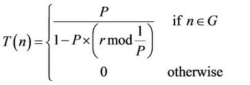
where P = the percentage of nodes that can become cluster heads (e.g., P = 0.05);
1/P = the number of subintervals in an interval;
r = the current subinterval;
G = the set of nodes that have not been cluster heads yet in the current interval.
Using this threshold, a node can be a cluster head in any one of 1/P subintervals in an interval. At the first subinterval of an interval (r = 0), each node has a probability P to become a cluster head. The nodes that are cluster heads in the first subinterval cannot be cluster heads in the next (1/P – 1) subintervals of the same interval. Thus, the probability of attaining cluster headships by the remaining nodes increases. After the completion of 1/P subintervals, a new interval will start, and all the nodes are again eligible to become cluster heads.
Each node, which has chosen itself as a cluster head in the current subinterval, broadcasts an advertisement message to the rest of the nodes. The non-cluster-head nodes will choose the cluster to which it will belong in this subinterval. This decision is based on the received signal strength of the advertised message. Assuming symmetric propagation channels, the cluster head whose advertisements have been heard with the largest signal strength will be selected by a non-cluster-head sensor node as its cluster head. In the case of a tie, a cluster head is chosen randomly.
3.2. Mathematical Models
There are some mathematical models available on LEACH. In [19], a simple mathematical model is proposed to compute the total energy dissipation in the sensor network for the transmission of a frame. Taking the derivative of the total energy it finds the optimum number of clusters, kopt as:

where N is the total number of sensor nodes, M is the dimension of the sensor area, dBS is the distance between cluster head and the base station,  and
and  are the amplifier energies.
In [47], a mathematical model is proposed to compute the total energy consumption in the sensor network during a single round. By taking the derivative of the total energy, it also finds the optimum number of clusters, kopt, as:

In [48], a mathematical model is proposed to calculate the total energy consumption in the sensor network during a single round. It also finds the optimum desired cluster head probability, popt as:
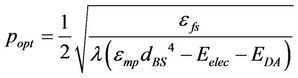
where λ is the intensity of homogeneous spatial Poisson process that indicates the sensor node density, Eelec is the electronic energy required for coding, modulation, filtering etc., and EDA is the energy required for data aggregation.
However, the lifetime of a sensor node is directly the inverse of its long run rate or expected rate of energy consumption. Therefore, in order to elongate network lifetime, the long run rate of energy consumption must be given more importance than other metrics (e.g., energy required to transmit one frame [47] or total energy consumption in an interval [48]). Moreover, none of these models consider the situation in which all the sensor nodes in the network can pick a random number higher than their respective thresholds and become a temporary follower. In this case, no sensor node will find any other node to choose as its cluster head under which it can keep its follower status. In this circumstance, every node is forced to directly communicate with the base station, i.e., all the sensor nodes will become a one-member cluster head. The complete mathematical model proposed in [49-51] incorporates all these factors.
In [50], Heinzelman’s First Order Radio Model [19,52] is used as the energy model and the Renewal Reward Process [50,53] is used as the underlying stochastic process to calculate the long run rate of energy consumption. It defines the following parameters in the model:
P = the desired percentage of cluster heads;
S = the number of subintervals in an interval, therefore s = 1/P;
Ph = the probability of becoming cluster head of a follower node at the start of any subinterval;
 = the probability of becoming cluster head of a cluster head node at the start of a subinterval in the next interval;
Φ0 = the probability of becoming cluster head of a sensor node at the start of any subinterval;
T(n) = the currently considered threshold value;
N = the total number of sensor nodes in the network;
a × b = the area of the rectangular coverage area.
According to the Renewal Reward Theorem, the rate of reward will be:
 (1)
(1)
where R is the reward and X is the cycle length. The model proposed in [50] considers the energy consumed by the sensor as the reward and the difference between two consecutive subintervals in which a sensor node becomes cluster head as the cycle.
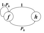
The model considers different state transition diagrams for a sensor node between two states while changing the subinterval in an interval and between two states while changing the subinterval as well as the interval to compute E(X). Figure 2 shows those state transition diagrams.
Using these state transition diagrams, the probability of becoming a cluster head, Φ0, at the start of any subinterval is calculated as follows:
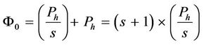 (2)
(2)
where Ph = P + (1 – P)N. Here, P contributes to the probability of becoming cluster head by choosing a random number less than the threshold and (1 – P)N is the probability of becoming a one-member cluster head in the case of choosing a random number not less than the threshold with no candidate cluster head found in the network.
After a number of steps, the long run rate of energy consumption is calculated as:
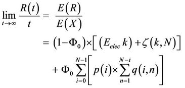 (3)
(3)
where,

 (a)
(a) (b)
(b)
Figure 2. State transition of a node while (a) Changing subinterval without changing the interval; (b) Changing subinterval as well as changing the interval.
Here, Eelec is the energy required per bit to run the circuitry in transmitter or receiver, EDA is the energy required for data aggregation,  is the energy constant for the radio transmission of a follower node,
  is the energy constant for the radio transmission of a cluster head node, k is the number of bits in a message, λ is the path loss exponent, dBS is the distance between the cluster head and the base station, and pa is the percentage of the circular area (centered at a follower and with a radius equal to the distance to a cluster head) falls within the sensor area. As we cannot get any closed form for the derivative of Equation (3), we can get the optimal percentage of the cluster heads by plotting the value of the long run rate of energy consumption from the equation.
3.3. Limitations
This algorithm introduced a fairly simple strategy which is more efficient than the direct transmission and the minimum-transmission-energy (MTE) protocol that chooses the route to minimize the transmitter’s energy. However, it has some limitations:
· LEACH always wants to achieve an even distribution of energy consumption, which might not be rational. Residual energies in different nodes do not remain the same after a significant amount of time of operation. Nodes with higher residual energy should get preference to be elected as cluster heads. Otherwise, longer network stability cannot be ensured.
· LEACH assigns all sensor nodes equal probability to become cluster heads. However, if a sensor node with very low residual energy is chosen to be cluster head, then it may quickly run out of energy. Therefore, there must be some sort of constraint to discount the sensor nodes having very low residual energy during the choice of cluster heads to prolong their lifetime. There is no such constraint in LEACH.
A number of variants have already been proposed for LEACH to overcome its limitations. Some of them are briefly summarized in the following section.
3.4. LEACH Variants
SEP [17] is a variant of LEACH that elects cluster heads based on weighted probabilities according to the residual energy of the sensor nodes. It assumes that a percentage of the sensor nodes is deployed with higher energy resources and studies the impact of such heterogeneity of the nodes based on their energy levels. It follows the underlying synchronization approach used in LEACH. In addition, it considers the variation in the residual energy assuming two types of nodes—normal and advanced.
SEP assumes m fractions of the nodes are advanced nodes, which have α times energy than that of the normal nodes. As a result, it assumes n(1 + αm) number of virtual normal nodes in the network. It extends the number of subintervals from 1/P to (1+ αm)/P in an interval. The objective of this extension is to elect a normal node once and an advanced node (1 + α) times as the cluster head in an interval. The probability equation to become a cluster head has been modified. In fact, two different equations are used for the normal and the advanced nodes. The weighted election probabilities for the normal and the advanced nodes are pnrm and padv respectively. Their equations are as follows:

and
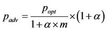
where popt is the optimal probability of a node to become a cluster head. It also uses two different equations for the threshold. One for the normal nodes called T(snrm) and the other for the advanced nodes called T(sadv). T(snrm) and T(sadv) are calculated as follows:
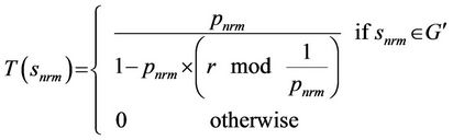

where G′ is the set of normal nodes that have not become cluster heads yet within the last 1/pnrm subintervals and G″ is the set of advanced nodes that have not become cluster heads yet within the last 1/padv subintervals in an interval.
SEP does not make any attempt to enhance the network stability. Besides, in SEP, the percentage of cluster heads is optimized based on the energy consumption in an interval. However, this value should be optimized on the basis of the long run rate or expected rate of energy consumption for achieving the higher network stability period. Finally, this work introduced the heterogeneity to LEACH in terms of two levels of residual energy. However, during the life cycle of the network the different levels of the residual energies may exist which will not be covered by only two types.
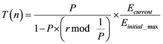
Deterministic Cluster Head Selection (DCHS) [18] introduces the heterogeneity to LEACH in terms of all levels of residual energy. It considers the residual energies of the sensor nodes in order to manage rational power consumption throughout the network. It exactly follows the underlying mechanism of LEACH. It only changes the equation of the threshold value to incorporate the residual energy in the cluster head selection process as follows:
where  is the current energy and
  is the initial energy of the node. The other parameters have the same definitions as of LEACH.
After a significant amount of time of operation, the residual energies of the sensors generally become very low, and then this threshold value will be very small. This can result in a situation where all the live sensors become one-member cluster head. In this case, the energy consumption rate will be very high. To break this stuck condition, another modified equation of the threshold value has been proposed as:
where rs is the number of consecutive rounds in which a node has not been a cluster head.
DCHS uses a random value for the percentage of cluster heads like LEACH. Therefore, it does not consider the optimal value of this parameter. Besides, it does not suggest any optimum value for rs. Finally, it did not attempt any improvement to enhance the network stability.
There are some other variants of LEACH in addition to these approaches. LEACH-C [19] is a centralized variant to cluster sensor nodes based on their positions. In this approach, the base station selects cluster heads to get uniformly-distributed clusters. In LEACH-C, sensor nodes detect their current locations using a GPS (Global Positioning System) receiver or any other technique. It precludes those sensor nodes whose residual energy is below the average residual energy from attaining cluster headship. The base station selects the cluster heads from the remaining nodes using the simulated annealing algorithm [54]. The base station also selects corresponding followers for the clusters while selecting the clusters and cluster heads, and the base station broadcasts a message into the network informing these selections.
This algorithm minimizes the total sum of squared distances between all the non-cluster-head nodes and the corresponding closest cluster head node. Thus, it minimizes the amount of energy required to transmit data to the cluster head nodes by the non-cluster-head nodes. However, the base station selects the cluster heads based on their positions and the average residual energy in the network. Therefore, like LEACH, the individual residual energy in each sensor node has little impact on the cluster head selection process in LEACH-C. This centralized algorithm also suffers from non-scalability. Besides, incorporating a GPS receiver or similar device in the sensor nodes increases sensor node cost. Finally, it did not attempt any improvement to enhance the network stability.
Another variant of LEACH, Adaptive Cluster Head Selection [20], assumes that a sensor node knows its distance from another sensor node by observing the signal strengths in the received messages. At first, this approach randomly selects cluster heads following LEACH. Next, it reselects the cluster heads considering the distance between each cluster head and the sensor nodes farthest from the cluster heads. The reselection is done in order to distribute the cluster heads uniformly in the network. This technique completely ignores the relative residual energy of each sensor node in the network while selecting the cluster heads. Besides, it did not make any attempt to enhance the network stability.
In summary, none of the research mentioned in this section makes any attempt to improve the network stability. Moreover, none of them investigate the applicability of relay nodes in a WSN during the clustering of sensor nodes the network. Therefore, in the next section, we propose a novel technique, Dynamic Clustering with Relay Nodes (DCRN), to improve network stability using relay nodes.
4. Dynamic Clustering with Relay Nodes (DCRN)
In this section, we propose a new algorithm to cluster sensor nodes in a network to improve network stability in terms of the death of the first sensor node. We follow the underlying approach of LEACH. In LEACH, each sensor node is given equal chance to get the cluster headship and thus its lifetime depends solely on its own residual energy. Therefore, a sensor node with low residual energy dies within a short period. However, there may be some other sensor nodes alive after its death. If that sensor node with low residual energy could exploit the residual energies of other high-energy live sensor nodes, then it would live longer. Therefore, we should choose cluster heads according to the residual energies to increase the stability period of a WSN. Moreover, deployment of relay nodes ensures the availability of high-energy sensor nodes in the network. Therefore, we should ensure the high probability of becoming cluster heads for these nodes. Besides, if no cluster head is found by a non-cluster head node, then the nearest relay node should be chosen as its default cluster head to avoid the situation of being a one-member cluster head. Finally, sensor nodes with very low residual energies should be excluded from choices of probable cluster heads to maximize their lifetimes. We present four heuristics to achieve these goals. We illustrate our complete clustering algorithm DCRN in detail after describing these heuristics. We also adapt the mathematical model derived in [50] for DCRN and incorporate the heuristics accordingly.
4.1. Heuristics
We propose four heuristics for DCRN in this subsection. The first two heuristics basically attempt to choose cluster heads according to relative residual energies of sensor nodes. The third heuristic attempts to avoid one member cluster headship for those sensor nodes that cannot discover any cluster heads in the network. The fourth heuristic provides a safeguard for low energy sensor nodes from becoming cluster heads. We describe these heuris tics as follows:
Heuristic 1: Energy consumption of a cluster head node is higher than that of a follower node. Therefore, sensor nodes with higher residual energy should be elected as cluster heads. In the original LEACH algorithm, network lifetime is divided into disjoint and discrete intervals that are again divided into some subintervals. If a LEACH node becomes a cluster head in a subinterval, it cannot become a cluster head again in any of the subsequent subintervals of the same interval. However, if a sensor node with higher residual energy can attain cluster headship again in other subintervals of the same interval, then a sensor node with lower residual energy can escape from being a cluster head. In that case, the lifetime of this lower energy sensor node will increase by indirect utilization of residual energy of the higher energy sensor node. For this reason, we make the subintervals completely memory-less and eliminate the use of the separate set of nodes that have not been cluster heads yet in the current interval. With this modification, the probability of becoming a cluster head of a sensor node in a subinterval does not depend on its status in the previous subintervals. This heuristic provides a fair increase in the network stability period. We have to consider more proportionate use of the residual energies to obtain further enhancement of the network stability period. Therefore, we adopt our next heuristic to ensure more proportionate use of the residual energies.
Heuristic 2: We can expect a higher stability period of a sensor network if we increase the probability of sensor nodes with higher residual energies becoming cluster heads. We should consider the relative residual energy of a sensor node to determine whether it is with higher residual energy or not. For this reason, we judge the relative residual energy of a sensor node while selecting it as a cluster head.
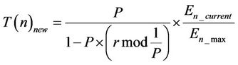
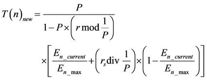
DCHS [18] attempts to exploit the relativity of residual energy of a sensor node by modifying the calculation of threshold value. This method multiplies the threshold equation of LEACH by the ratio between the current energy and the initial energy of a sensor node. This modification allows us to consider the relativity of residual energy. However, this relativity is obtained with respect to the own initial energy of a sensor node. We should consider the relativity with respect to the whole network as the deployment of relay nodes and the heterogeneity of initial energy results in significant variation in initial energies of different sensor nodes. Therefore, we further modify the equation of the threshold and take the multiplying factor as the ratio between current energy and maximum initial energy over the network. The changed equation of the threshold will be:
 (4)
(4)
where Ecurrent is the current energy of a sensor node and  is the maximum initial energy all over the network. Ecurrent is measured at the beginning of each interval, whereas
  is measured prior to the deployment. This equation is used by all sensor nodes in the network. Therefore, if the residual energy of a relay node becomes lower than that of a normal sensor node, then the probability of the relay node becoming the cluster head will also be lower than that of the normal node. This phenomenon ensures a longer time interval before the death of the first node in network.
The modified threshold value may become very small after a long duration of operation. The small value may inhibit sensor nodes from becoming cluster heads. DCHS proposes another modification in equation of the threshold to adapt this situation. However, we do not need any further modification as our next heuristic will take care of this situation.
Heuristic 3: A sensor node becomes a follower when it picks a random number greater than its threshold, T(n), and it finds a candidate cluster head node. Therefore, the node will become a cluster head even by choosing a random number greater than its threshold if it does not find any candidate cluster head. It may result in two situations—if there is no candidate cluster head in the network or the node cannot successfully receive any of the advertisement messages from the candidate cluster heads. In either case, attaining the cluster headship by the node significantly increases its energy consumption rate. Therefore, we propose a heuristic to impose the choice of the nearest relay node as cluster head in case no candidate cluster head is found. This heuristic completely eliminates the situation where all nodes in the network become one-member cluster heads, and thus it attains significant improvement in the overall energy consumption rate of the network.
Heuristic 4: The stochastic nature of attaining cluster headship imposes a nonzero probability of becoming a cluster head to all live nodes. However, a node with low residual energy will quickly run out of energy if it attains cluster headship. Therefore, we propose our last heuristic to utilize a minimum threshold value on the residual energy to make a node eligible for attaining the cluster headship. A node with residual energy less than the threshold is completely ignored during the cluster head selection. This heuristic guarantees an elongated lifetime for nodes with low residual energy and thus increases the stability period of the network.
Now, we present a complete algorithm for DCRN exploiting all these heuristics in the next subsection.
4.2. DCRN Algorithm
In the DCRN algorithm, we divide the lifetime of the network into some discrete and disjoint equal length intervals in DCRN. Here, each sensor node operates in these intervals. The intervals are maintained using clock synchronization [55-58]. Each interval has three consecutive phases—advertisement, cluster-setup, and steadystate phase. The DCRN algorithm, depicted in Figure 3, runs independently in each sensor node in each interval. The phases are executed as follows:
1) Advertisement Phase: Each relay node broadcasts a RELAY_EXPOSUE message in this phase. Besides, all the sensor nodes independently decide whether or not to become cluster heads. To make this decision, each node computes the threshold, T(n) using Equation 4. Then, it picks a random number and compares the random number with the threshold. If the random number is less than the threshold, then it becomes a cluster head and broadcasts the HEAD_EXPOSURE message.
2) Cluster Set-Up Phase: Each non-cluster-head sensor node independently attempts to choose its cluster head in this phase. It may encounter two cases during the attempt:
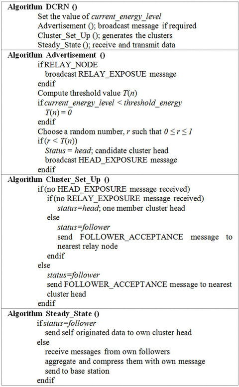
Figure 3. Algorithm for dynamic clustering with relay nodes (DCRN).
· CASE 1: It receives one or more copies of HEAD_ EXPOSURE messages from other candidate cluster head nodes. In this case, the sensor node attempts to become a follower of the nearest candidate cluster head node and sends a FOLLOWER_ACCEPTANCE message to that node. Here, the sensor node chooses the cluster head node with maximum signal strength as the nearest cluster head [20].
· CASE 2: It does not experience any arrival of the HEAD_EXPOSURE message from other sensor nodes. In this case, the sensor node tries to be a follower of the nearest live relay node. If it does not find any live relay node, it becomes a one member cluster head.
3) Steady-State Phase: In this phase, the followers send data to their corresponding cluster heads. The cluster heads accumulate, aggregate, and compress the received data with its own data. Cluster heads send the aggregated and compressed data to the base station. The duration of steady-state phase is significantly longer than the summation of the durations of the advertisement and cluster set-up phases in order to minimize the cluster establishment overhead.
4.3. Mathematical Model of DCRN
The difference between the underlying mode of operations of LEACH and DCRN arises because of the new heuristics. The last two heuristics make changes only in the threshold value (T(n)). This change merely affects the probability of becoming a cluster head of a follower node at the start of any subinterval (Ph). Otherwise, there is no impact of these two heuristics on Equation (3), which is the latest mathematical formulation of LEACH.
On the other hand, Heuristic 1 of our new clustering algorithm makes the subinterval completely memory-less. For this heuristic, the first state transition diagram of Figure 2 is no longer applicable. However, Φ0 is formulated from the weighted combination of the two state transition diagrams of Figure 2 in the mathematical model of LEACH. Therefore, the formulation of Φ0 needs to be changed in the mathematical model of DCRN. With the introduction of Heuristic 1, any sensor node can become a cluster head irrespective of its status in the previous sub interval. Therefore, the probability of becoming a cluster head of a follower node at the start of any subinterval (Ph) will no longer differ from the probability of becoming a cluster head of a sensor node at the start of any subinterval (Φ0). As a result, we get a new formulation of Φ0 as Φ0 = Ph in the changed mathematiccal model of DCRN.
On the other hand, the third heuristic imposes followership to a node that would be a candidate for becoming a one-member cluster head according to LEACH, if it receives any RELAY_EXPOSURE message. Therefore, this heuristic lowers the probability of becoming a cluster head by reducing the probability of becoming a onemember cluster head. We formulate the new probability of becoming a cluster head, Φ0 as:
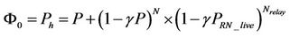 (5)
(5)
where  is the probability that at least one relay node is live, Nrelay is the total number of relay nodes, and γ is the probability of successful transmission that reflects environmental effects as well as interference in the network.
With this change, we can use Equation (3) as the mathematical model of DCRN. We compare this mathematiccal model with that of LEACH by simulation results in the next section. We also analyze the efficiency of DCRN in that section.
5. Simulation Results
We conduct our simulation runs on a randomly deployed wireless sensor network. Our simulation program is written in Visual C++. In this section, we first describe our network settings along with various parameters used in the energy rate calculation. Then, we compare the mathematical models of DCRN with that of LEACH. Finally, we evaluate network stability in DCRN with that of LEACH and the best variant of LEACH, DCHS.
5.1. Network Settings
We use the network settings as shown in Figure 4 in our simulation runs. The settings are as follows:
· The total number of sensor nodes in the network is 100.
· The dimensions of the sensor area are 200 × 200, having the base station at (600, 100). We consider all dimensions and distance values in terms of meters.
· The sensor nodes are uniformly distributed over the sensor area. However, relay nodes are placed to ensure equal coverage for all of them. In our experiment, the optimal number of relay nodes is four, which is found by the mathematical model in Section 5.2. These nodes are placed at (50, 50), (50, 100), (100, 50), and (100, 100).
· Each sensor node is initially equipped with a battery of 1 - 5 Joules. Sensor nodes have initial energy uniformly distributed over this range and the distribution is shown in Figure 5.
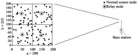
Figure 4. Network settings: uniformly distributed sensor nodes with a base station.
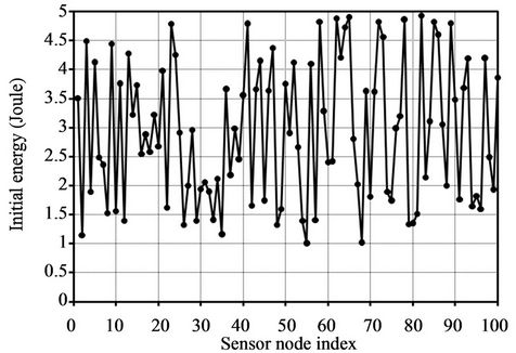
Figure 5. Initial energies of sensor nodes: uniformly distributed in range [1J, 5J].
We use the following parameters [2] in the simulation runs for verification of the mathematical models and in subsequent analysis:
· The amount of energy per bit to run sensor node circuitry, Eelec, is 5 × 10⁻⁸;
· The value of energy constant, Єamp, for radio transmission, is 1 × 10⁻¹⁰;
· The number of data packets generated during each subinterval by a sensor node is normally distributed in the range of [0, 50], with a mean value of 25. We applied the Box-Muller transformation [59] to achieve this normal distribution from the uniform distribution of the built-in rand() function in visual C++;
· Each data unit contains 8 bits of data;
· The probability that a message successfully arrives at its destination is 90% (i.e., γ = 0.9).
5.2. Verification of the Mathematical Model
We first plot the long run rate of energy consumption versus the percentage of cluster heads from the mathematical model of LEACH in Figure 6. We compute the values using Equation (3). We calculate the value of the probability of becoming a cluster head of a sensor node at the start of any subinterval (Φ0) using Equation (2), and it must not exceed 1. Here, if the percentage of cluster heads (P) exceeds 0.61, then the value will exceed 1. In order to avoid this, we plot the graph against the percentage of cluster heads up to 0.61. According to the graph:
· The energy consumption rate initially decreases very sharply with the increase of the percentage of cluster heads.
· There is an optimal point for which the energy consumption rate is the lowest. After this point, the energy consumption rate increases with the increase of the percentage of cluster heads. In our simulation result, the optimal point for LEACH is (0.045, 0.0005912). The optimal point is explicitly shown in Figure 6.
We also plot the long run rate of energy consumption versus the percentage of heads from the mathematical model of DCRN in Figure 7. We compute the values using Equation (3) like LEACH. However, we calculate the value of Φ0 using Equation (5) rather than Equation (2). Here, we plot the graph against the percentage of cluster heads up to 1 as the value of Φ0 remains within 1 for these values.
The graph in Figure 7 exhibits almost the same trends found in the graph in Figure 6. The energy consumption rate initially decreases very sharply with the increase of the percentage of cluster heads and after an optimal point, the energy consumption rate increases with the increase of the percentage of cluster heads. In Figure 7, the optimal point for DCRN is (0.035, 0.004022). There are two implications of this point:
· This point indicates that the optimal percentage of cluster heads is 3.5%. It also indicates the optimal percentage of relay nodes as we deploy the relay nodes to primarily act as cluster heads.
· The optimal point provides a 32% lower long run rate of energy consumption than the optimal point for LEACH found in Figure 6. This improvement arises due to the first and third heuristics, as only these heuristics modify the mathematical model.
Next, we evaluate the network stability of DCRN against that of LAECH and its best variant. [18] claims that DCHS improves the network stability period by 30% over LEACH, whereas [17] claims that SEP does the improvement over LEACH by 26%. These two are the most improved LEACH variants claimed so far. For this reason, we take the Deterministic Cluster Head Selection [18] as the best LEACH variant instead of SEP in our
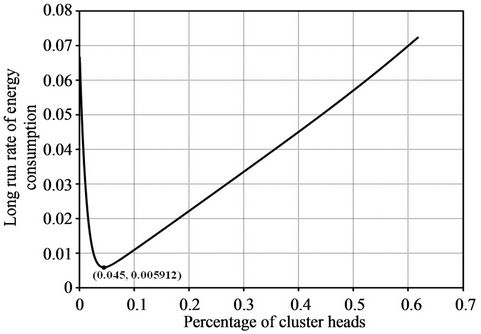
Figure 6. Long run rate of energy consumption against different percentage of cluster heads according to the mathematical model of LEACH.
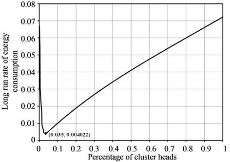
Figure 7. Long run rate of energy consumption against different percentage of cluster heads according to the mathematical model of DCRN.
performance comparison.
We utilize an optimal percentage of cluster heads for all the algorithms under evaluation. We have already found the optimal percentages of cluster heads as 0.045 and 0.035 for LEACH and DCRN respectively from the mathematical models. The optimal percentage of cluster heads for the LEACH variant is empirically found as 0.05 in [49]. We evaluate all these techniques at their optimal percentage of cluster heads. Our evaluation is based on three parameters:
1) Data rate of a sensor node;
2) Position of the base station; and 3) Initial energy of the relay nodes.
In the evaluation process, we measure network lifetime in terms of duration before death of the first sensor node as well as duration before death of half of the sensor nodes. The former one is generally termed as First Node Dies (FND) and the later one is termed as Half of the Nodes Die (HND). We plot 15 points of FND and HND for each of the three metrics. We take the average of 100 simulation passes for each of those points. For the first point in each case, we use similar sensor node placements to those already described in Section 5.1. We vary the corresponding metric by a certain constant value to obtain each subsequent point. We present our findings obtained from the evaluation below.
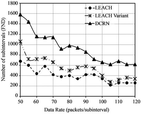
5.2.1. Data Rate of a Sensor Node
In the initial network settings, the number of data packets generated by a sensor node in a subinterval is symmetrically and normally distributed in the range of 0 to 50, with the mean of 25. We conduct 15 simulation runs varying this range. We change the upper limit of the range from 50 packets with a step of 5 packets in each simulation run. We plot the values of network stability periods in terms of First Node Dies (FND) in Figure 8(a) and the values of Half of the Nodes Die (HND) in Figure 8(b). There is a significant improvement in FND for DCRN over LEACH and its variant in Figure 8(a). The average improvement over LEACH and its variant is 137% and 74% accordingly. On the other hand, Figure 8(b) indicates that HNDs of DCRN, LEACH, and the LEACH variant are comparable. Here, we obtain moderate average improvement over LEACH and its variant of 19% and 11% accordingly.
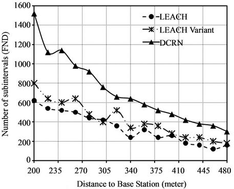
5.2.2. Position of the Base Station
In the initial network settings, the base station is located at (300, 100). Therefore, the distance of the base station from the center of the network area is 200 meters. We conduct 15 simulation runs varying this distance. We change the position of the base station in the first dimension from 300 meters with a step of 20 meters in each simulation run. We plot the values of network stability
 (a)
(a)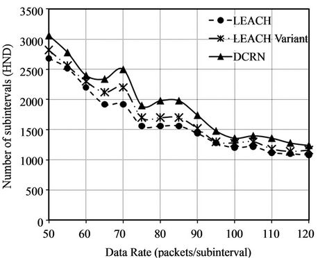 (b)
(b)
Figure 8. Comparison of FND and HND for different data rates. (a) Improved network stability period in terms of First Node Dies (FND); (b) Comparable number of subintervals before Half of the Nodes Die (HND).
periods in terms of FND in Figure 9(a) and the values of HND in Figure 9(b). There is a significant improvement in FND for DCRN over LEACH and its variant in Figure 9(a). The average improvement over LEACH and its variant is 117% and 70% accordingly. On the other hand, Figure 9(b) indicates that HNDs of DCRN, LEACH, and the LEACH variant are comparable. Here, we obtain moderate average improvement over LEACH and its variant of 15% and 10% accordingly.
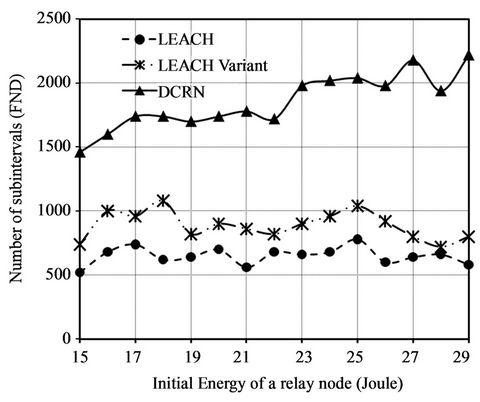
5.2.3. Initial Energy of the Relay Nodes
In the initial network settings, the initial energy of relay nodes is 15 Joule. We conduct 15 simulation runs varying this initial energy. We change the initial energy from 15 Joules with a step of 1 Joule in each simulation run. We plot the values of network stability periods in terms of FND in Figure 10(a) and the values of HND in Figure
 (a)
(a)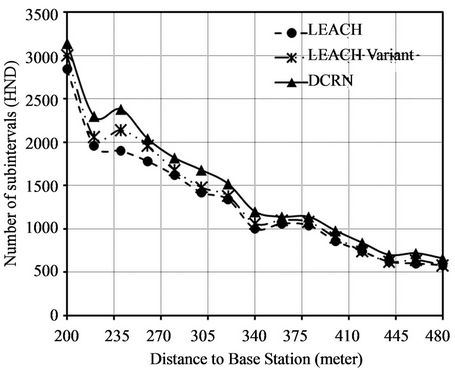 (b)
(b)
Figure 9. Comparison of FND and HND for different position of base station. (a) Improved network stability period in terms of First Node Dies (FND); (b) Comparable number of subintervals before Half of the Nodes Die (HND).
10(b). There is a significant improvement in FND for DCRN over LEACH and its variant in Figure 10(a). The average improvement over LEACH and its variant is 188% and 112% accordingly. This high average value is obtained due to higher improvement with the increasing initial energy of relay node. The upward trend of the graph for DCRN with increasing value of initial energy in Figure 10(a) indicates this scenario. On the other hand, Figure 10(b) indicates that HNDs of DCRN, LEACH, and the LEACH variant are comparable. Here, we obtain moderate average improvement over LEACH and its variant of 23% and 15% accordingly.
These values clearly indicate that DCRN provides significantly higher time before the death of the first node in comparison to LEACH and its variants irrespective of the data rate of the sensor node, the position of the base station, or the initial energy of relay nodes. The perform-
 (a)
(a)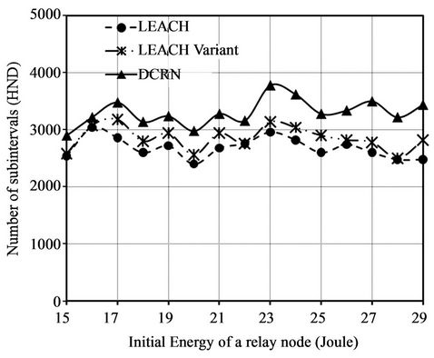 (b)
(b)
Figure 10. Comparison of FND and HND for different initial energy of relay nodes. (a) Improved network stability period in terms of First Node Dies (FND); (b) Comparable number of subintervals before Half of the Nodes Die (HND).
ance of DCRN becomes even better with an increase of initial energy in relay nodes. Moreover, in all cases, DCRN also provides moderate improvement of HND over LEACH and its variant.
6. Future Work
We propose DCRN for sensor nodes with similar transmission and sensing ranges. In our future work, we will attempt to enhance DCRN for sensor nodes with varying transmission and sensing ranges. In addition, we will also attempt to enhance DCRN for multi radio sensor nodes, which are now emerging in recent research [60]. Finally, we will try to incorporate multi-hop clustering in DCRN to further optimize energy efficiency.
7. Conclusion
Clustering techniques have the inherent potential to effectively balance the energy consumption throughout a wireless sensor network to improve the stability of the network. Deployment of relay nodes can enhance the potential to a great extent if they are considered in a suitable way during the clustering mechanism. In this paper, we propose a novel dynamic, self-organizing, and adaptive technique DCRN to cluster sensor nodes in WSN with relay nodes to exploit the potential. We do not make any assumption in DCRN such that only relay nodes attain cluster headships, whereas such assumption is enforced in the previous work. Therefore, DCRN does not suffer from any of the limitations of lower fault tolerance or reduced network stability due to the assumption.
To devise DCRN, we use four heuristics with proper justifications. We present a complete mathematical formulation for DCRN exploiting that of LEACH. We present the improvement achieved in DCRN using the mathematical model. Besides, we evaluate the stability period of DCRN with that of LEACH and its best variant through simulation results. The results suggest that DCRN achieves significant improvement in network stability under different circumstances.
REFERENCES
- I. Dietrich and F. Dressler, “On the Lifetime of Wireless Sensor Networks,” ACM Transactions on Sensor Networks (TOSN), Vol. 5, No. 1, 2009, pp. 1-39. doi:10.1145/1464420.1464425
- W. B. Heinzelman, A. P. Chandrakasan and H. Balakrishnan, “Energy Efficient Communication Protocol for Wireless Microsensor Networks,” Proceedings of the 33rd Annual Hawaii International Conference on System Sciences, Maui, 1-7 January 2000. doi:10.1109/HICSS.2000.926982
- J. Han and K. Micheline, “Data Mining Concepts and Techniques,” Morgan Kauffman, Waltham, 2001.
- S. Basagni, “Distributed Clustering Algorithm for ad-hoc Networks,” Proceedings of International Symposium on Parallel Architectures, Algorithms and Networks, Perth/ Fremantle, 23-25 June 1999, pp. 310-315. doi:10.1109/ISPAN.1999.778957
- S. Banerjee and S. Khuller, “A Clustering Scheme for Hierarchical Control in Multi-Hop Wireless Networks,” Proceedings of Twentieth Annual Joint Conference of the IEEE Computer and Communications Societies, Anchorage, 22-26 April 2001, pp. 1028-1037.
- M. Gerla, T. J. Kwon and G. Pei, “On Demand Routing in Large Ad Hoc Wireless Networks with Passive Clustering,” Proceeding of Wireless Communications and Networking Conference, Chicago, 23-28 September 2000, pp. 100-105.
- C. R. Lin and M. Gerla, “Adaptive Clustering for Mobile Wireless Networks,” IEEE Journal on Selected Areas in Communications, Vol. 15, No. 7, 1997, pp. 1265-1275. doi:10.1109/49.622910
- J. Kamimura, N. Wakamiya and M. Murata, “Energy-Efficient Clustering Method for Data Gathering in Sensor Networks,” Proceedings of Workshop on Broadband Advanced Sensor Networks, San Jose, 25-29 October 2004, pp. 31-36.
- J. J. Y. Leu, M.-H. Tsai, T.-C. Chiang and Y.-M. Huang, “Adaptive Power Aware Clustering and Multicasting Protocol for Mobile Ad Hoc Networks,” International Conference on Ubiquitous Intelligence and Computing, Wuhan, 3-6 September 2006, pp. 331-340.
- S. Lindsey and C. S. Raghavendra, “PEGASIS: PowerEfficient Gathering in Sensor Information Systems,” Aerospace Conference Proceedings, Big Sky, 9-16 March 2002, pp. 1125-1130. doi:10.1109/AERO.2002.1035242
- L. Li, S. Dong and X. Wen, “An Energy Efficient Clustering Routing Algorithm for Wireless Sensor Networks,” The Journal of China Universities of Posts and Telecommunications, Vol. 3, No. 13, 2006, pp. 71-75. doi:10.1016/S1005-8885(07)60015-6
- Y. Sangho, H. Junyoung, C. Yookun and H. Jiman, “PEACH: Power-Efficient and Adaptive Clustering Hierarchy Protocol for Wireless Sensor Networks,” Computer Communications, Vol. 30, No. 14-15, 2007, pp. 2842-2852. doi:10.1016/j.comcom.2007.05.034
- S. Ghiasi, A. Srivastava, X. Yang and M. Sarrafzadeh, “Optimal Energy Aware Clustering in Sensor Networks,” SENSORS Journal, Vol. 7, No. 2, 2002, pp. 258-269.
- H. Chan and A. Perrig, “ACE: An Emergent Algorithm for Highly Uniform Cluster Formation,” Lecture Notes in Computer Science, Vol. 2920, 2004, pp. 154-171.
- O. Younis and S. Fahmy, “Distributed Clustering in AdHoc Sensor Networks: A Hybrid, Energy-Efficient Approach,” Proceedings of IEEE the 23rd Conference of the IEEE Communications Society, Hong Kong, 7-11 March 2004, pp. 366-379.
- J. Y. Cheng, S. J. Ruan, R. G. Cheng and T. T. Hsu, “PADCP: Poweraware Dynamic Clustering Protocol for Wireless Sensor Network,” International Conference on Wireless and Optical Communications Networks, Banglore, 11-13 April 2006.
- G. Smaragdakis, I. Matta and A. Bestavros, “SEP: A Stable Election Protocol for Clustered Heterogeneous Wireless Sensor Networks,” Proceedings of the International Workshop on SANPA, Boston, 22 August 2004.
- M. Haase and D. Timmermann, “Low Energy Adaptive Clustering Hierarchy with Deterministic Cluster-Head Selection,” The 4th International Workshop on Mobile and Wireless Communications Network, Stockholm, 9-11 September 2002, pp. 368-372.
- W. B. Heinzelman, A. P. Chandrakasan and H. Balakrishnan, “An Application-Specific Protocol Architecture for Wireless Microsensor Networks,” IEEE Transactions on Wireless Communications, Vol. 1, No. 4, 2002, pp. 660- 670. doi:10.1109/TWC.2002.804190
- C. Nam, H. Jeong and D. Shin, “The Adaptive Cluster Head Selection in Wireless Sensor Networks,” IEEE International Workshop on Semantic Computing and Applications, Incheon, 19-21 September 2008, pp. 147-149.
- A. Giridhar and P. R. Kumar, “Maximizing the Functional Lifetime of Sensor Networks,” The Fourth International Symposium on Information Processing in Sensor Networks, Los Angeles, 25-27 April 2005, pp. 5-12.
- X. Wang, W. Gu, S. Chellappan, K. Schosek and D. Xuan, “Lifetime Optimization of Sensor Networks under Physical Attacks,” Proceedings of IEEE International Conference on Communications, Seoul, 16-20 May 2005, pp. 3295-3301.
- H. Zhang and J. C. Hou, “Maximizing α-Lifetime for Wireless Sensor Networks,” International Journal of Sensor Networks, Vol. 1, No. 1, 2006, pp. 64-71. doi:10.1504/IJSNET.2006.010835
- V. Rai and R. N. Mahapatra, “Lifetime Modeling of a Sensor Network,” Proceedings of Design, Automation and Test in Europe, Munich, 7-11 March 2005, pp. 202- 203.
- M. U. Ilyas and H. Radha, “Increasing Network Lifetime of an IEEE 802.15.4 Wireless Sensor Network by Energy Efficient Routing,” IEEE International Conference on Communications, Istanbul, 11-15 June 2006, pp. 3978- 3983. doi:10.1109/ICC.2006.255703
- L. Shi, A. Capponi, K. H. Johansson and R. M. Murray, “Sensor Network Lifetime Maximization via Sensor Trees Construction and Scheduling,” The Third International Workshop on Feedback Control Implementation and Design in Computing Systems and Networks, Annapolis, 6 June 2008.
- P. Berman, G. Calinescu, C. Shah and A. Zelikovsky, “Power Efficient Monitoring Management in Sensor Networks,” IEEE Wireless Communication and Networking Conference, Atlanta, 21-25 March 2004, pp. 2329-2334.
- D. Brinza and A. Zelikovsky, “DEEPS: Deterministic Energy-Efficient Protocol for Sensor Networks,” International Workshop on Self-Assembling Wireless Networks, Las Vegas, 19-20 June 2006, pp. 261-266.
- A. Aung, “Distributed Algorithms for Improving Wireless Sensor Network Lifetime with Adjustable Sensing Range,” Master’s Thesis, Georgia State University, Atlanta, 2007.
- S. G. Akojwar and R. M. Patrikar, “Improving Life Time of Wireless Sensor Networks Using Neural Network Based Classification Techniques with Cooperative Routing,” International Journal of Communications, Vol. 1, No. 2, 2008, pp. 75-86.
- Y. Chen, Q. Zhao, V. Krishnamurthy and D. Djonin, “Transmission Scheduling for Sensor Network Lifetime Maximization: A Shortest Path Bandit Formulation,” IEEE International Conference on Acoustics, Speech and Signal Processing, Toulouse, 14-19 May 2006.
- K. Dasgupta, K. Kalpakis and P. Namjoshi, “Improving the Lifetime of Sensor Networks via Intelligent Selection of Data Aggregation Trees,” Proceedings of the Communication Networks and Distributed Systems Modeling and Simulation Conference, Orlando, 19-23 January 2003.
- H. Kang and X. Li, “Power-Aware Sensor Selection in Wireless Sensor Networks,” Proceedings of the 5th International Conference on Information Processing in Sensor Networks, Nashville, 19-21 April 2006.
- M. Cardei and D. Du, “Summary on Improving Wireless Sensor Network Lifetime through Power Aware Organization,” Seminar on Theoretical Computer Science, 2005.
- J. Park and S. Sahni, “An Online Heuristic for Maximum Lifetime Routing in Wireless Sensor Networks,” IEEE Transactions on Computers, Vol. 55, No. 8, 2006, pp. 1048-1056. doi:10.1109/TC.2006.116
- J. Chang and L. Tassiulas, “Maximum Lifetime Routing in Wireless Sensor Networks,” IEEE/ACM Transactions on Networking, Vol. 12, No. 4, 2004, pp. 609-619. doi:10.1109/TNET.2004.833122
- P. Djukic and S. Valaee, “Maximum Network Lifetime in Fault Tolerant Sensor Networks,” IEEE Global Telecommunications Conference, Saint Louis, 28 November-2 December 2005, pp. 3106-3111.
- M. Cardei, J. Wu, M. Lu and M. O. Pervaiz, “Maximum Network Lifetime in Wireless Sensor Networks with Adjustable Sensing Ranges,” International Conference on Wireless and Mobile Computing, Networking and Communications, Montreal, 13-16 August 2005, pp. 438-445.
- K. Kalpakis, K. Dasgupta and P. Namjoshi, “Efficient Algorithms for Maximum Lifetime Data Gathering and Aggregation in Wireless Sensor Networks,” Computer Networks, Vol. 42, No. 6, 2003, pp. 697-716. doi:10.1016/S1389-1286(03)00212-3
- R. Madan and S. Lall, “Distributed Algorithms for Maximum Lifetime Routing in Wireless Sensor Networks,” IEEE Transactions on Wireless Communications, Vol. 5, No. 8, 2006, pp. 2185-2193. doi:10.1109/TWC.2006.1687734
- Y. T. Hou, Y. Shi, H. D. Sherali and S. F. Midkiff, “Prolonging Sensor Network Lifetime with Energy Provisioning and Relay Node Placement,” The Second Annual IEEE Communications Society Conference on Sensor and Ad Hoc Communications and Networks, Santa Clara, 26- 29 September 2005, pp. 295-304. doi:10.1109/SAHCN.2005.1557084
- X. Han, X. Cao, E. L. Lloyd and C.-C. Shen, “Fault-Tolerant Relay Node Placement in Heterogeneous Wireless Sensor Networks,” The 26th IEEE International Conference on Computer Communications, Anchorage, 6-12 May 2007, pp. 1667-1675.
- W. Zhang, G. Xue and S. Misra, “Fault-Tolerant Relay Node Placement in Wireless Sensor Networks: Problems and Algorithms,” The 26th IEEE International Conference on Computer Communications, Anchorage, 6-12 May 2007, pp. 1649-1657.
- B. Hao, J. Tang and G. Xue, “Fault-Tolerant Relay Node Placement in Wireless Sensor Networks: Formulation and Approximation,” Proceedings of IEEE Workshop High Performance Switching and Routing, Phoenix, 19-21 April 2004, pp. 246-250.
- E. L. Lloyd and G. Xue, “Relay Node Placement in Wireless Sensor Networks,” IEEE Transactions on Computers, Vol. 56, No. 1, 2007, pp. 134-138. doi:10.1109/TC.2007.250629
- W. Wang, V. Srinivasan and K.-C. Chua, “Using Mobile Relays to Prolong the Lifetime of Wireless Sensor Networks,” Proceedings of the 11th ACM International Conference on Mobile Computing and Networking, Cologne, August 28-September 2, 2005, pp. 270-283.
- J. C. Choi and C. W. Lee, “Energy Modeling for the Cluster-Based Sensor Networks,” Proceedings of the Sixth IEEE International Conference on Computer and Information Technology, Seoul, 20-22 September 2006, p. 218.
- S. Selvakennedy and S. Sinnappan, “An Energy-Efficient Clustering Algorithm for Multihop Data Gathering in Wireless Sensor Networks,” Journal of Computers, Vol. 1, No. 1, 2006, pp. 40-47. doi:10.4304/jcp.1.1.40-47
- A. B. M. A. Al Islam, “A Novel Approach to Cluster Heterogeneous Sensor Network (CHSN),” M.Sc. Engineering Thesis, 2009, pp. 31-41.
- A. B. M. A. A. Islam, C. S. Hyder, M. H. Kabir and M. Naznin, “Finding the Optimal Percentage of Cluster Heads from a New and Complete Mathematical Model on LEACH,” Wireless Sensor Network, Vol. 2, No. 2, 2010. pp. 129-140. doi:10.4236/wsn.2010.22018
- A. B. M. A. A. Islam, C. S. Hyder, M. H. Kabir and M. Naznin, “Stable Sensor Network (SSN): A Dynamic Clustering Technique for Maximizing Stability in Wireless Sensor Networks,” Wireless Sensor Network, Vol. 2, No. 7, 2010, pp. 538-554. doi:10.4236/wsn.2010.27066
- K. Dasgupta, K. Kalpakis and P. Namjoshi, “An Efficient Clustering-Based Heuristic for Data Gathering and Aggregation in Sensor Networks,” Proceedings of the IEEE Wireless Communications and Networking Conference, New Orleans, 16-20 March 2003, pp. 1948-1953.
- D. Song, “Probabilistic Modeling of Leach Protocol and Computing Sensor Energy Consumption Rate in Sensor Networks,” Technical Report, 22 February 2005.
- T. Murata and H. Ishibuchi, “Performance Evaluation of Genetic Algorithms for Flowshop Scheduling Problems,” Proceedings of 1st IEEE Conference Evolutionary Computation, Orlando, 27-29 June 1994, pp. 812-817.
- B. Sundararaman, U. Buy and A. Kshemkalyani, “Clock Synchronization for Wireless Sensor Networks: A Survey,” Ad Hoc Network, Vol. 3, No. 3, 2005, pp. 281-323. doi:10.1016/j.adhoc.2005.01.002
- Q. Li and D. Rus, “Global Clock Synchronization in Sensor Networks,” Proceedings of IEEE Conference on Computer Communications, Hong Kong, 7-11 March 2004, pp. 564-574.
- L. Meier, P. Blum and L. Thiele, “Internal Synchronization of Drift-Constrained Clocks in Ad-Hoc Sensor Networks,” Proceedings of the 5th ACM International Symposium on Mobile Ad Hoc Networking and Computing, Tokyo, 24- 26 May 2004, pp. 90-97.
- M. L. Sichitiu and C. Veerarittiphan, “Simple, Accurate Time Synchronization for Wireless Sensor Networks,” Proceedings of IEEE Wireless Communications and Networking Conference, New Orleans, 16-20 March 2003, pp. 1266-1273.
- G. E. P. Box and M. E. Muller, “A Note on the Generation of Random Normal Deviates,” The Annals of Mathematical Statistics, Vol. 29, No. 2, 1958, pp. 610-611.
- [61] A. B. M. A. A. Islam, M. S. Hossain, V. Raghunathan and Y. C. Hu, “Backpacking: Deployment of Heterogeneous Radios in High Data Rate Sensor Networks,” Proceedings of IEEE International Conference on Computer Communications and Networks, Maui, 31 July-4 August 2011, pp. 1-8.