Int'l J. of Communications, Network and System Sciences
Vol.4 No.1(2011), Article ID:3700,12 pages DOI:10.4236/ijcns.2011.41008
A Parametric Colored Petri Net Model of a Switched Network
1Department of Information Technology, International Humanitarian University, Odessa, Ukraine 2Department of Switching Systems, Odessa National Academy of Telecommunications, Odessa, Ukraine
E-mail: zsoftua@yahoo.com, tishtri@rambler.ru
Received February 26, 2010; revised March 30, 2010; accepted April 2, 2010
Keywords: Switched Network, Colored Petri Net, Parametric Model, Network Response Time
Abstract
A parametric Colored Petri net model of the switched Ethernet network with the tree-like topology is developed. The model’s structure is the same for any given network and contains fixed number of nodes. The tree-like topology of a definite network is given as the marking of dedicated places. The model represents a network containing workstations, servers, switches, and provides the evaluation of the network response time. Besides topology, the parameters of the model are performances of hardware and software used within the network. Performance evaluation for the network of the railway dispatcher center is implemented. Topics of the steady-stable condition and the optimal choice of hardware are discussed.
1. Introduction
The performance evaluation of networks is a significant task especially for real-time applications such as technological processes and traffic control. The complexity of modern networks makes pure analytical methods difficult, for instance, the theory of Markovian processes or the theory of queueing networks. For this purpose, ad hoc simulating systems are developed [1]. These simulating systems are implemented as extensions to programming languages; they are narrowly specialized, relaying strongly on the peculiarities of the application field.
Petri nets constitute a universal language for asynchronous systems and processes description. Colored Petri nets [2] implemented in CPN Tools [3] allow the representation of plain colored nets as well as timed and hierarchical nets. Since for the description of elements the programming language CPN ML close to standard ML is used, colored net is a very powerful and convenient tool for various systems specification. The range of projects with CPN Tools application includes telecommunication protocols verification, vehicles control and the planning of military operations. For the investigation of the models’ behavior, a simple simulation of processes’ dynamics is used as well as the construction and analysis of the state space. But the state space construction is useful for such tasks as protocols verification [4]. In performance evaluation, we are interested in the statistical characteristics of models’ behavior.
For these purposes CPN Tools proposes a wide range of implemented random functions, for instance, uniformly, exponentially distributed etc. Besides standard facilities for the accumulation of statistical information, special measuring fragments of Petri net model [5] are used.
The earlier presented model of switched network [6] was supplied with measuring fragments for the network response time calculation [5] and features for dynamic maintenance of switching tables [7]. The model is constructed of such components as submodels of switch, workstation, server, and measuring workstation. But at the modeling of each new network, we have to assemble the top page out of submodels according to the given topology of network. In the present work we propose the parametric model, which is invariant with respect to topology. An arbitrary topology of the tree-like structure with an arbitrary number of switches and terminal devices is represented as data in the form of the marking for two dedicated places of Petri net. The constructed model was used for performance evaluation of the switched network for a railway dispatcher center supplied with GID-Ural [8] CAM software.
The remainder of this paper is organized as follows. Section 2 gives an overview of switched Ethernet and presents examples of networks. Section 3 discusses facilities of Colored Petri nets and describes the parametric model of switched Ethernet with the tree-like topology. Section 4 presents the way, in which the parameters of the model may be calculated on the characteristics of hardware and software. Section 5 describes the process of model’s behavior simulation. Section 6 contains the results of performance evaluation for the network of a railway dispatcher center. Section 7 summarizes the paper and gives directions for the application of obtained results.
2. Overview of Switched Networking
In the modern epoch of the entirely switched full-duplex Ethernet, the procedures of Carrier Sense Multiply Access with Collision Detection (CSMA/CD), stipulated by the standard IEEE 802.3, are losing their urgency. A microsegmented network [9] uses point-to-point connections only; moreover, the full-duplex mode provides separate channels for independent frames’ transmission in the both directions. Even backpressure procedures are not required if IEEE 802.3x Advanced Flow Control (AFC) is implemented. Each channel of the full-duplex connection may be either free or busy with the transmission of a frame. AFC uses two messages: “suspend transmission” and “resume transmission”. It is implemented in the model with special labels of a channel’s availability. Practically, an entirely switched Ethernet works without collisions providing maximal throughput per each channel equaling 10 Mbps for classical Ethernet IEEE 802.3, 100 Mbps for Fast Ethernet IEEE 802.3u and 1 Gbps for Gigabit Ethernet IEEE 802.3z. We may represent in our models segments, which a few hosts are attached to, for instance, via a hub but it’s a historical necessity only. Such devices as hubs are transparent for switched network and do not have a separate representation in models.
According to standards, the frames of useful capacity from 46 to 1500 bytes are transmitted. The frame header contains source and destination addresses and the actual length (or type) of the frame. 6-bytes Media Access Address (MAC) is used. The key element of a network is a switch of frames. As the rule, the majority of modern switches work in store-and-forward mode. At the receiving of a frame the switch stores it in the internal buffer and then forwards the frame to the output port, the target device is attached to. For making the decision regarding the output port number, the switch uses a switching table, each record of which constitutes a pair: MAC-address and port number. Either dynamic or static tables are used. Recently static tables are applied for networks with high requirements for secrecy only. The static table is entered manually by the administrator of a network. For the construction of dynamic table, the switch only listens to network passively looking for new MAC-addresses. If the destination is unknown, then the switch forwards the frame to all its ports. The records of the table are erased periodically to provide correspondence to the actual structure of the network. In the present work we consider static tables; the influence of dynamic switching on the performance was investigated in [7].
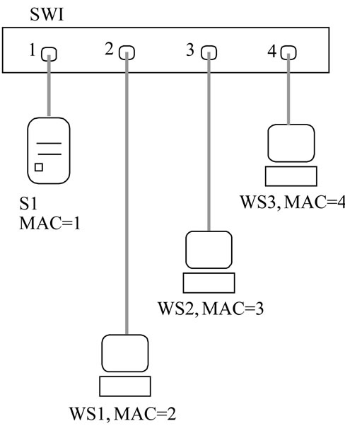
Most widespread topologies of Ethernet are the star shown in Figure 1(a) and the tree shown in Figure 1(b). Star topology is the simplest; it is constituted by single switch (SWI) as well as a stack of switches logically considered as a single switch. To each port of switch only terminal devices are attached. In the tree-like topology, there are connections between switches, which are named by uplinks. In such a network the frame passes a few switches on its way to a target device and in the general case each switch has to know all the MAC-addresses of the network. In this study, we do not consider more complex topologies with duplicated paths between devices because these topologies require modeling the spanning tree procedures stipulated by standard IEEE 802.1 D.
To represent realistic traffic we consider an information system, which uses the network. As a rule, for realtime applications such as technological processes control, there is the primary information system. For instance, Figure 1 represents the networks of railway dispatch centers, supplied with CAM system GID-Ural [8]. On the peculiarities of traffic, we distinguish workstations (WS), which generates requests and servers (S), which executes requests and send responses to workstations. We consider only two-way handshake “request-response” in such an interaction but more complicated protocols may be implemented also.
3. Model of Switched Network
3.1. The Overview of Colored Petri Nets
Petri net [4] is a bipartite directed graph supplied with dynamic elements named by tokens. The first part of nodes is named by places and is drawn as circles (ellipses), the second part—by transitions drawn as bars. Tokens are represented with dots situated inside places. They move through net modeling processes. First colored Petri nets [2] were suggested to distinguish tokens
 (a)
(a)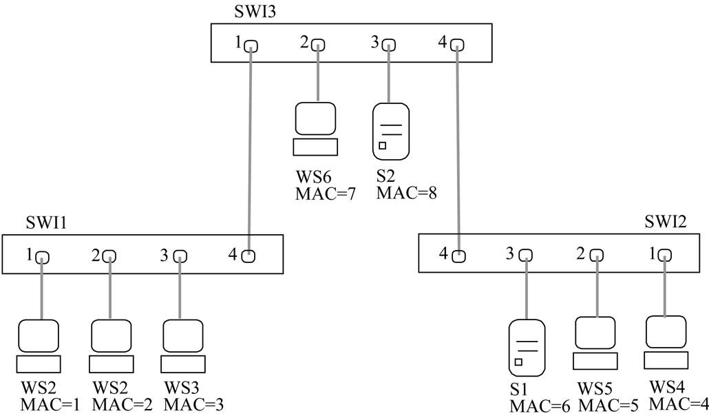 (b)
(b)
Figure 1. Topologies of network. (a) LAN1; (b) LAN2.
as natural numbers. For a finite set of numbers a vivid its representation via colors was possible.
CPN Tools [3] uses special kind of colored Petri nets [2] in which tokens are elements of an abstract data type but data types are traditionally named by colors. For description of colors and attributes of places, transitions and arcs CPN ML language is used. The tokens of a place (marking of a place) are represented by multiset; an element belongs to a multiset with a given multiplicity (in a definite number of copies). The multisets are represented by expressions of the following form: k1`e1 ++ k2`e2 ++ … ++kl`el, where ki is the multiplicity of element ei.
A place possesses a name, color, initial marking and a current marking. A transition possesses a name, guard and time delay. The input arc of a transition has an inscription defining the pattern for token extraction. The output arc of a transition has an inscription defining the pattern for creation of tokens. The guard constitutes a predicate, which defines the condition for transition’s firing.
To model times, special timed multisets of the form e@t are used. It means that token e may be used only after instance t of the model time. In such a notation, @ + d represents the delay with the duration d. Delays may be assigned to transitions as well as to individual tokens.
The dynamics of the net consists in moving the tokens as the result of transitions’ firings. Transition is fireable (permitted) if there are tokens in its input places, which satisfies both the inscriptions of arcs and the guard. At firing, transition extracts tokens from its input places and puts new tokens, constructed according to the rules of output arcs’ inscriptions, into its output places. All the output tokens are delayed with the transition’s firing delay.
Besides CPN Tools colored Petri nets were implemented in such well known software as Design/CPN, Helena, Miss-RdP and applied successfully in such areas as networking, protocols’ verification, trains’ traffic control, military operations planning, vehicles control, satellite communications and aeronautics.
3.2. Description of Model
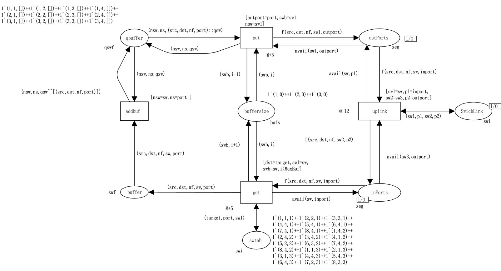
A parametric colored Petri net model of a switched network is represented in Figures 2-6. The initial parameters correspond to the network structural scheme shown in Figure 1(b). The main page of the model (Figure 2) employs four subpages corresponding to switches SW (Figure 3), workstations WS (Figure 4), servers S (Figure 5), and measuring fragments MEA (Figure 6); declarations are represented in Table 1.
In the comparison with the previously presented model [5], the parametric model (Figure 2) is invariant with respect to the networks’ topology. Each page of the model represents all the devices of the same type. For instance, the page SW reflects all the switches of a given network. The solution was obtained on the base of a special tag, which accomplishes merely each element of the model. The tag uniquely defines the segment of a network, which target devices are attached to, with two fields: the number of switch and the number of a switch’s port. The only exception is a segment, which connects a pair of switches. Such a segment has duplicated notation with respect to the upper and lower switches, which it is attached to. The following elements of model are labeled with tags: frames, records of switching table and tokens of a segments’ availability.
For a detailed description of the model let us consider the descriptions of colors, variables, constants and func-
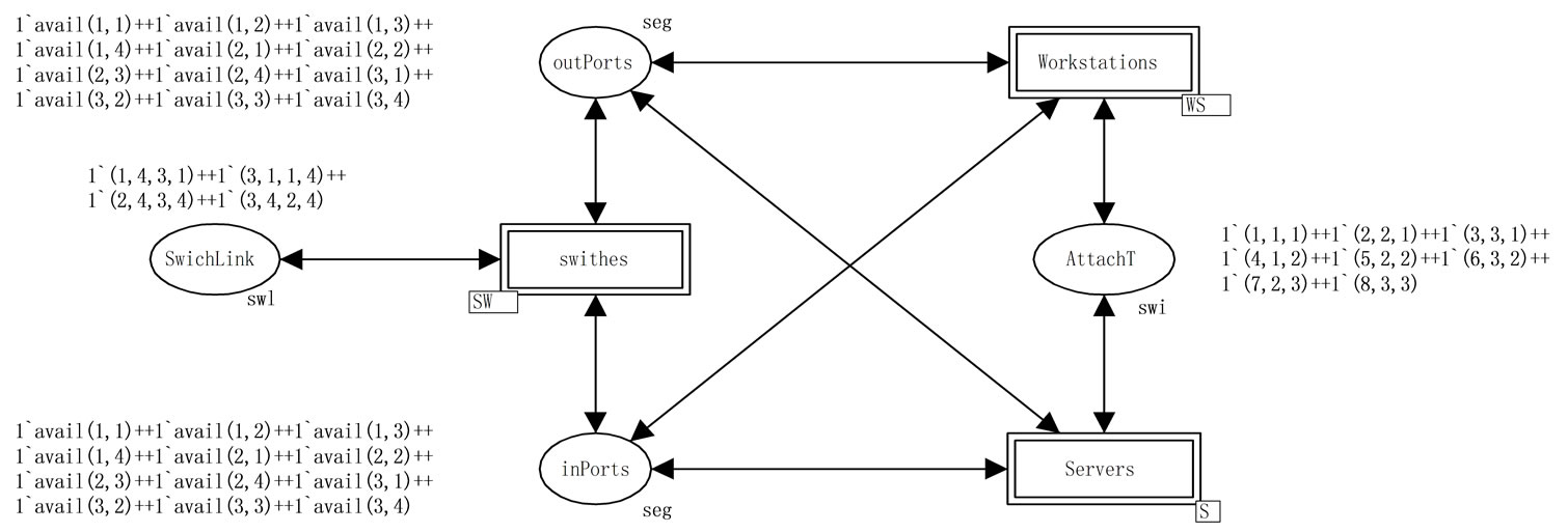
Figure 2. The main page of the parametric model.
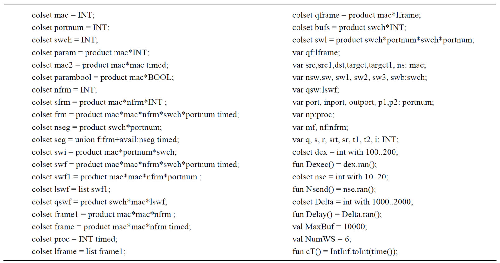
Table 1. Descriptions of colors, variables and functions.
tions, represented in Table 1. Media Access Control addresses (mac), port numbers (portnum), switch numbers (swch), frames’ sequential numbers (nfrm) are represented with integer type. We abstract from the content of a frame and consider only its header. The frame is represented by color frm, which contains destination and source MAC-addresses, sequential number of request used for the calculation of network response time and the tag with number of switch and number of port. It should be mentioned, that only the destination and source addresses correspond to the real fields of an Ethernet frame’s header, remaining variables are artificially added for the purposes of parametric model’s construction and measurement. Auxiliary types frame, frame1 are used inside submodel of server (S); they do not contain the tag with switch and port number. The only difference between them consists in the option timed.
For the adequate modeling of frames’ transmission through Ethernet segments, color seg is introduced. It constitutes a union of color frm and unit color avail. Really, if we do not consider collisions, then each channel of a segment may be either available for transmission or busy with the transmission of a frame. In this parametric model all the segments are represented with a pair of places: outPorts, inPorts. These separate places reflect full-duplex mode of data transmission. The places are named with respect to the switch, which the terminal devices are attached to. For instance, place inPorts models transmission of frames from servers and workstations to switches, whereas place outPorts models the transmission of frames from switches to workstations and servers. That is why labels avail bears the tags with number of switch
and number of port. In the initial marking we have a separate label for each segment of network. Before transmission of a frame into the segment, each device is waiting for the corresponding avail label and removes this label replacing it by frame. At the acceptance of the frame by device, it is replaced by the corresponding avail label. The described procedure guarantees that not more than one frame is being transmitted in each segment at the same time.
The page SW (Figure 3) represents all the switches. Note that, segments, which connect switches, have a pair of labels avail with the respect to each switch. To process this special case the transition uplink is introduced. It provides the transformation of the segment’s number and moves the frame from the place outPorts for source switch to the place inPorts for destination switch. Place SwitchLink contains the information about the connections among switches represented with color swl. This color includes definitions for the both ends of connection: the number of the switch and the number of the port.
The color swi is used for the description of static switching tables for all the switches of the network. It consists of usual fields of switching table such as MAC-address and port’s number accomplished with the tag containing the number of switch. All the switching tables are represented with the marking of a single place swtab. Using records from this place switch assigns the output port’s number for arrived frame via the transition get. Then frame is allocated in the internal buffer of switch represented with place qbuffer. Each token in this place models the queue to a given port of a given switch. The record of the queue is described with color swf1 (swf), whereas the queue is represented with the color qswf. The frame is moved to the output segment of switch via transition put. Place buffersize counts the number of occupied slots of frames’ buffer for each switch. The limits of buffer sizes are checked in the guard of transition get.
The page WS (Figure 4) represents all the workstations, whereas the page S (Figure 5) represents all the servers. It’s implemented in such a way that each host listens for the frame with its destination address only in the segment, which it is attached to. A simple description of network’s topology is situated in the place AttachT. Color swi is used for assignment of Ehternet segment for each MAC-address; segment is given by the pair: number of switch and number of port. It should be noted that, together with the marking of the place SwitchLink place AttachT gives the complete information about network’s topology. Place AttachT is used either at listening a segment for receiving a frame via transitions receive* (receiveWS, receiveS) or at uttering a frame into segment via transitions send* (sendWS, sendS).
We consider a simple two-way handshake as the protocol of client-server interaction. The workstation sends a request; the server executes the request and sends an answer. Delays between the client’s requests are represented with uniformly distributed random function Delay(); time of request execution by server is represented
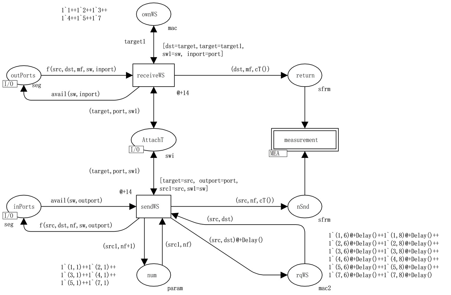
Figure 4. Parametric model of workstations (WS).
with function Dexec(). We consider a request consisting of a single frame and the response consisting of a random number of frames represented with function Nsend(). Moreover, we suppose that each server has a few processors defined by the marking of place processor. This place contains the number of processors for a given MAC-addresses of servers.
Let us consider the trace of client-server interaction to study the model more thoroughly. Place rqWS defines the activity of workstations pointing the servers, which they require. Color mac2 is used to define the pairs: MACaddress of workstation, MAC-address of server. After uttering the frame of request into the segment via transition sendWS the pair is frozen on the duration given with function Delay(). Through switches the frame arrives into segment, which the target server is attached to. The server reads the frame via the transition receiveS and puts it into the input queue of the server via transition addqreq. Each token of the place qrequest represents a queue to the corresponding server. After the execution of the request via transition exec, obtained reply consisting of Nsend() frames is situated into place reply. Note that, at construction the frames of reply, we change the positions of the source and destination addresses in the frame’s header to provide the backward transmission from server to required workstation. All the replies are moved into output queues represented with place qreply. Each token in place qreply corresponds to the output queue of a given server. Then frames are transmitted into segment, which the server is attached to, via transition sendS. Segment is determined on the base of information about network’s topology situated in place AttachT. Through switches the frame arrives into a segment, which the required workstation is attached to, and is accepted via transition receiveWS.
For the calculation of Network Response Time (NRT) we use the special measuring fragment of colored Petri net MEA (Figure 6). Elements of this fragment do not model any real software of hardware; they are used for the purposes of measurement only. For each pair of communicating server and workstation, we enumerate the requests via counters stored in place num. In the model representtation each frame bears the auxiliary information, which includes the described tag with the number of the segment as well as the ordinal number of request given by variable nf. The time of the requests uttering is stored in place nSnd. Color sfrm unites MAC-address of workstation, ordinal number of request and the model time of request. The frames of reply accomplished with the timestamps of arrival times are stored in place return. Transition IsFirst determines the first frame of the reply and launches the process of response times’ recalculation.
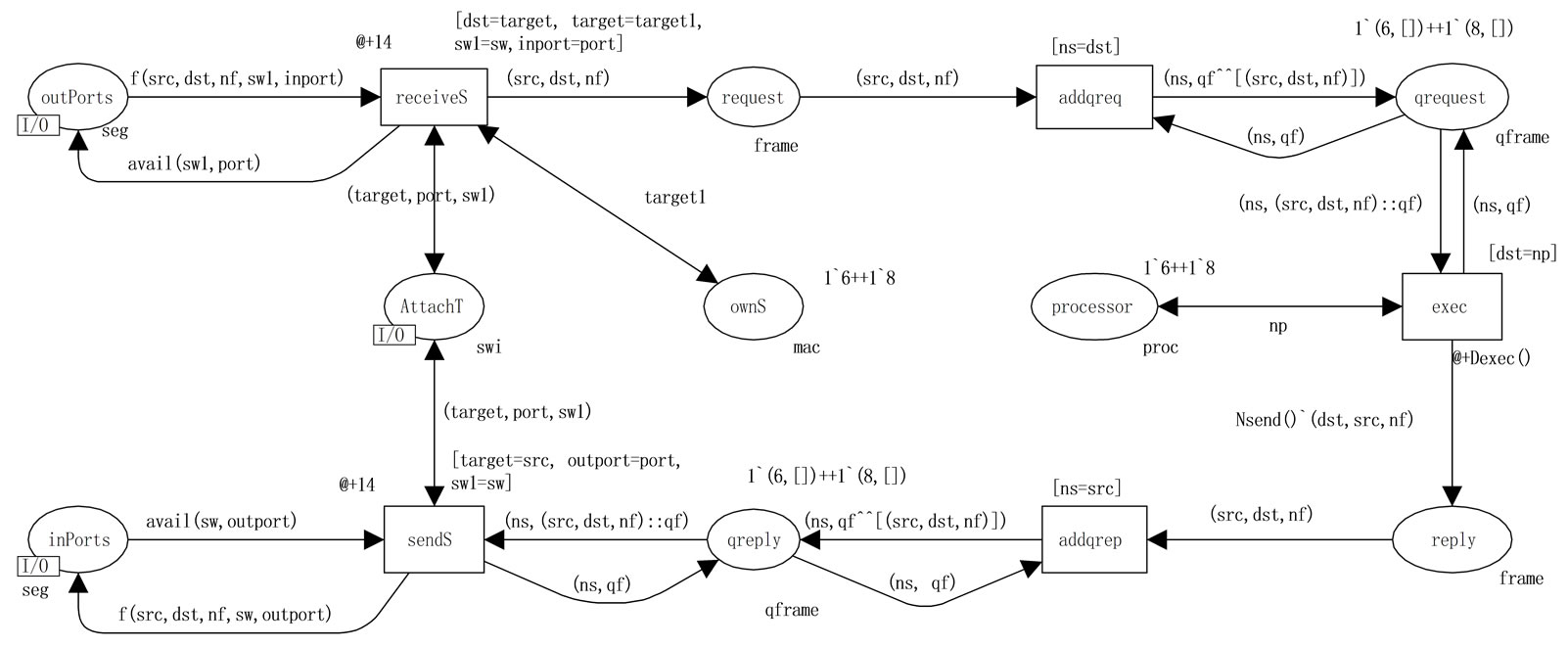
Figure 5. Parametric model of servers (S).
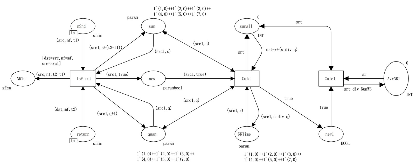
Figure 6. Measuring fragment for the network response time evaluation (MEA).
For debugging purposes response times for all the requests are stored in place NRTs. But we are interested especially in the average response times. The residuary part of the measuring fragment calculates the average response times for each workstation (place NRtime) via transition Culc and the total average response time for the entire network (place AvrNRT) via transition Culc1.
4. Parameters of Model
4.1. Topological Parameters
The primary information about the topology of networks is represented as the marking of places AttachT and SwitchLink. Place AttachT of color swi enumerates MACaddresses of terminal devices attached to each port of each switch. Note that, the hubs usage may be represented by a few MAC-addresses attached to the same port. Links between switches (uplinks) are represented by the marking of place SwitchLink with color swl. Color swl describes both ends of link as a pair: the number of switch and the number of port. For modeling convenience each link is described twice for each of the two possible directions of the frames’ transmission. For instance, for the network drawn in Figure 1(a) the marking of place SwitchLink would be empty and marking of place AttachT would be equal to: 1`(1,1,1) ++ 1`(2,2,1) ++ 1`(3,3,1) ++ 1`(4,4,1).
The switching tables constitute the secondary information about topology. All the switching tables of all the switches are represented with the marking of the same place swtab with color swi. Since each switch contains information about each known terminal device, there are a few records for a chosen MAC-address; the number of these records corresponds to the number of switches. For instance, for the network drawn in Figure 1(a) the marking of place swtab would be the same as the marking of place AttachT. Note that, for an arbitrary network with the star topology, the markings of places AttachT and swtab coincide and marking of place SwitchLink is empty.
Thus, places AttachT and SwitchLink contain the encoding of the network tree: leaves of the tree are mentioned in place AttachT while internal nodes (including the root) are mentioned in place SwitchLink.
4.2. Parameters of Hardware
We consider both the network hardware such as switches and network adapters, and the terminal hardware such as workstations and servers. For convenience we consider frames of maximal length with useful capacity of 1500 Kbytes and express parameters of the model with respect to this size of frame. In the data sheets of switches either performance in frames per second or in gigabits per second is written. For instance, switch Intel SS101TX4EU possesses the performance of about 10000 packets per second [10]. From this value we calculate the average time of one frame processing as 100 ms, which corresponds to the total delay of transitions get and put. An ideal performance of the network is defined by its standard, for instance the minimal time of 1500 byte frame transmission accounting for an additional size of header, preamble and standard delay between frames is equal to 123 ms for 100 Mbps Ethernet. Furthermore in calculations we use the total length of a frame equaling to 12304 bits. Real Ethernet adapters provide a lesser performance; an evaluation is presented in [10]. For instance, the card Intel Ether Express PRO/100+ provide actual performance in one direction about 92,1 Mbps; this corresponds to the delay about 140 ms. This value represents the delays of transitions send*, receive*.
Performances of workstations and servers have different influences on the parameters of the model. The performance of a workstation is not essential for the period of requests, which is determined mainly by the characteristics of information system and relays on slow by thousands times man-machine interaction. Therefore we consider the period of requests completely defined by parameters of an information system. The performance of a server has a direct influence on the time of a request’s execution. The average time of request execution (transition exec) may be either measured for each type of hardware on the test sequences of requests or calculated on the information about the number of abstract operations and performance. In both mentioned cases it relays on parameters of software and will be discussed in the next section.
Note that, the modeling system maintains time in its internal units MTU (Model Time Unit). Before modeling we have to express all the timed values in MTU using the scaling of times. As 1 MTU we may choose the smallest time value among all the parameters but for the purposes of future representation of faster devices it is appreciated to choose more little value. For instance, in the model shown in Figure 2, MTU is equal to 10 ms.
4.3. Parameters of Software
We consider as the primary such parameters of software as: the period of workstations’ requests, the average length of request, the average hardness of request’s execution, the average length of response. We study the CAM software GID-Ural [8] of trains’ traffic control. Since the period of requests depends weakly on the performance of hardware, we measure it directly in timed intervals as uniformly distributed random value given by function Delay() of range 20-40 ms or 2000-4000 MTU. The lengths of requests and responses primarily given with the number of bytes we measure in number of frames with maximal length; they are also represented as uniformly distributed random values. For instance, request length 1-1,5 Kb is represented with one frame, response length 15-30 Kb is represented with a random function Nsend() of range 10-20 frames.
We estimated the average time of request execution on test sequences of requests for the HP Brio server; it equals to 1-2 ms and it is represented in the model with the uniformly distributed random function Dexec() of the range 100-200 MTU. Moreover, the model reflects the information links between the workstation and the servers given by the table of workstations’ activity represented with the marking of place rqWS, which contain a token with the address of the workstation and the address of the server for each the interacting pair of terminal devices. In our example each workstation interacts with each server.
5. Simulation
For the debugging of models CPN Tools provides the step-by-step mode of simulation with visual displaying of all the events at the current moment of model time. Either one step or a given number of steps may be executed. It is assumed, that a step corresponds to an occurrence of an event. The next moment of model time is calculated according to the list of future events.
Let us consider the process of a request’s frame transmission from one of workstations to server and response's frames backwards from server to requested workstation. This delivery loop is the base one for the client-server systems. The initial state of the model is given by Figures 2-6. The current marking of places created on initial marking is shown inside green rectangles beside corresponding place; the number of tokens is written inside small circles. Clicking on these circles user can show or hide place’s marking. Note that according to the marking of place rqWS generated by random function Delay() initial moment of model time is equal to 2031.
For compact representation of the simulation process, we use the trace table (Table 2). This table describes states of model at each step. Note that the table contains only base elements of the model, which participate in the frames’ transmitting.
Frame (7,8,1) with request 1 of workstation WS6 (mac = 7) sent to server S2 (mac = 8) at step 1, has been delivered to server at 4th step and executed by server at 13th step; as the result 12 frames of reply have been generated. Beginning at 13th step the delivery of frames in the opposite direction is executed. At step 16 the first frame of the reply has been delivered to workstation WS6 and absorbed by transition receiveWS. It should be noticed, that Table 2 displays also others events taking place in the model. For instance, execution of the request of workstation WS5 (mac = 5) sent to server S2 at step 6.
Let us consider in detail the process of frames’ tags modification, since it is the base for the parametric model behavior comprehension. At step 1, tag of request’s frame (3,2) is created by transition sendWS according to network’s topology given by place AttachT: MAC address 7 is attached to port 2 of switch 3. After switching at step 3, tag (3,3) is assigned by transition put because target device with MAC address 8 is attached to port 3 of the same switch 3. Analogous assignment of tags is executed for reply’s frames at steps 13, 15 by transitions sendS, put. More complicated case constitutes the request of WS5 to server S2 because client and server are attached to different switches. Initial tag (2,2) is replaced by tag (2,4) at step 8 and then at step 9 is overwritten with tag (3,4) by transition uplink representing the transmission between switches 2 and 3; the frame is redirected from port 4 output channel of switch 2 to port 4 input channel of switch 3. The assignment of tag (3,3) at step 11 finishes the delivery of request to target device attached to port 3 of switch 3.
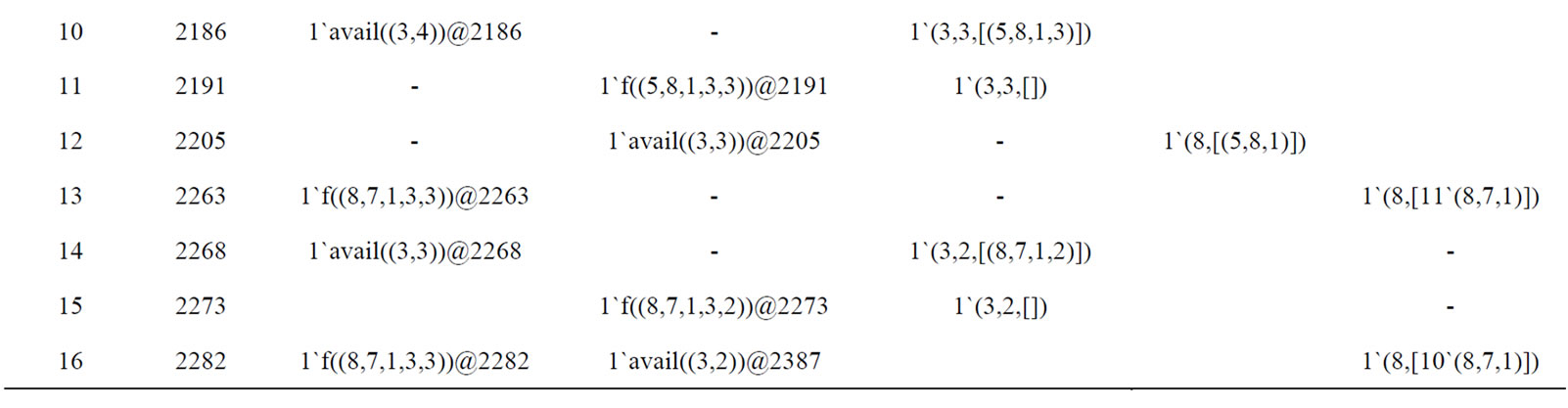
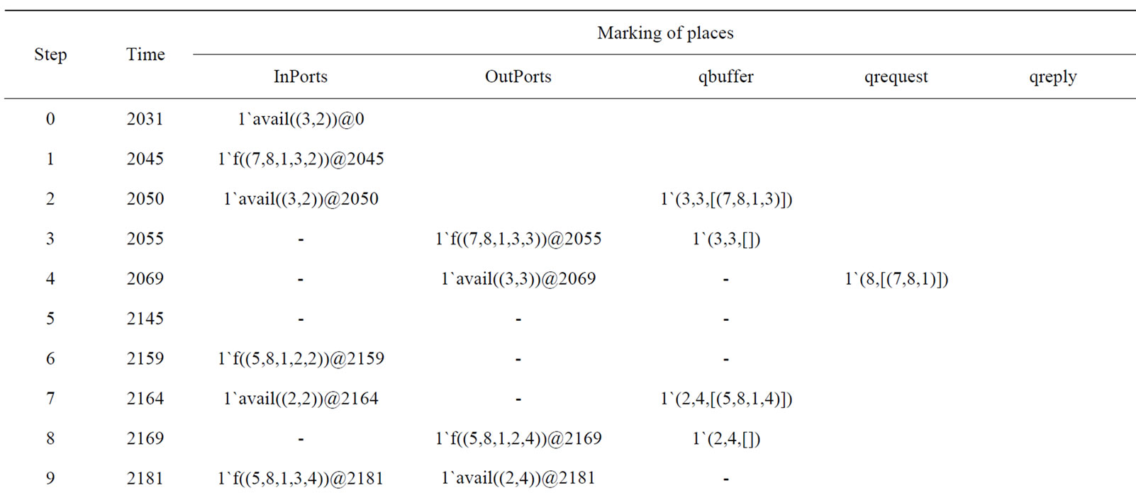
Table 2. Trace of model’s behavior.
As the trace table (Table 2) contains complete loop of client-server interaction for the pair of MAC addresses (7,8), let us consider the network response time (NRT) calculation. The time of request (2031) was saved in the place nSnd and the time of reply’s arrival (2273) is saved in place return; the sequential number of request is indicated by field nf of frame. After reply’s arrival, transition IsFirst recognizes the first frame of reply and starts the process of response time’s recalculation. Place Sum contains (7,242), that means: the sum of response times for workstation with MAC address 7 is equal to 242 (2273- 2031). Place quan contains (7,1): number of responded requests for workstation with MAC address 7 is equal to 1. Place new runs the recalculating of average NRT for each workstation by transition Calc, which are stored in place NRTime: (7,242). Note that, place AvrNRT contains inconsistent values only at startup interval of time before the arrival of responses for each workstation.
6. Performance Evaluation
For the debugging of models, CPN Tools proposes stepby-step simulation as well as automatic slow simulation with the visualization of Petri net dynamics for a specified number of steps. For the accumulation of statistical information, a special mode of fast simulation without visualization is used. It provides the consideration of huge enough intervals of real time.
6.1. Conditions for Steady-State Mode
The major question we are interested in is the existence of the steady-state mode. For the parameters of the model shown in Figure 2-6 we obtain the steady-state mode, which may be observed for instance using Table 3. After model time instance 100000 the value of NRT is stabilized and does not change any more. This interval corresponds to one and a half second of real time. Obtained network response time equaling to 392 MTU or about 4 ms satisfies the requirements of train traffic control [8].
Table 4 illustrates the absence of the steady-state mode for the 10 Mbps network. The value of NRT is growing in time. As we may easily conclude from the bottom row of the table, this is concerned with the growth of frames’ output queues in servers.
6.2. Evaluation of Characteristics
Furthermore we are investigating the behavior of the network in the steady-state mode. We are interested in the variations of NRT with respect to different network
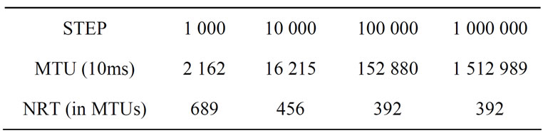
Table 3. Steady-state mode of network behavior.
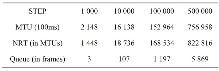
Table 4. Absence of steady-state mode for 10 Mbps network.
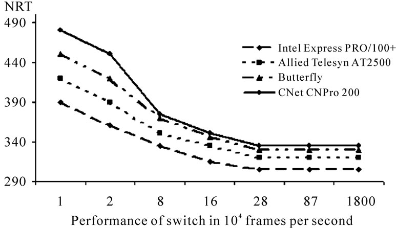
and computer hardware (Figure 7). In this study, we try four 100 Mbps network adapters Intel Express PRO/100+, Allied Telesyn AT2500, Butterfly, Cnet CNPro 200 with characteristics given in [10] as well as four servers HP Brio, Power Mac, SGI Origin, Sun Fire. Switches are estimated with two parameters: the performance in frames per second and size of buffer in Kb. The extreme ends of graphs in Figure 7(a) corresponds to Intel SS101TX4EU and 3Com Switch 4005, intermediate points represent switches of Cisco Catalist series.
Figure 7(a) shows that switches choice with performance greater than 28 104 frames per second, which corresponds to switch Catalist 2900XL, does not lead to a decrease of NRT. Figure 7(b) shows that only switches’ buffers lesser than 16Kb have influence on NRT. In Figure 7(c) the total influence of network hardware such as switches and network adapters on NRT is illustrated; the surface has the form of an inclined strip. Figure 7(d) contains the diagram, which illustrates the variation of NRT on servers’ hardware and number of processors. There is no merely difference between NRT for servers with more than two processors.
Constructed graphs may be applied for solving the task of the optimal network’s hardware choice. Two basic characteristics, such as NRT and the cost of hardware, may be considered either as the criteria or as the bound.
Note that, the results obtained with the parametric and nonparametric [5] models coincide but the parametric model does not require the editing of model structure for each given network: only the encoded network tree is put into places AttachT and SwitchLink.
7. Conclusions
A parametric Colored Petri net model of the switched Ethernet network with the tree-like topology was developed. The components of the network are workstations,
 (a)
(a)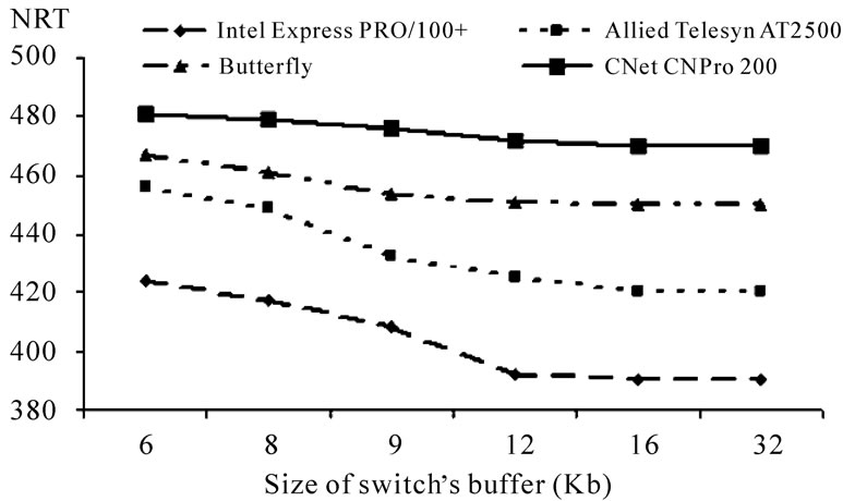 (b)
(b)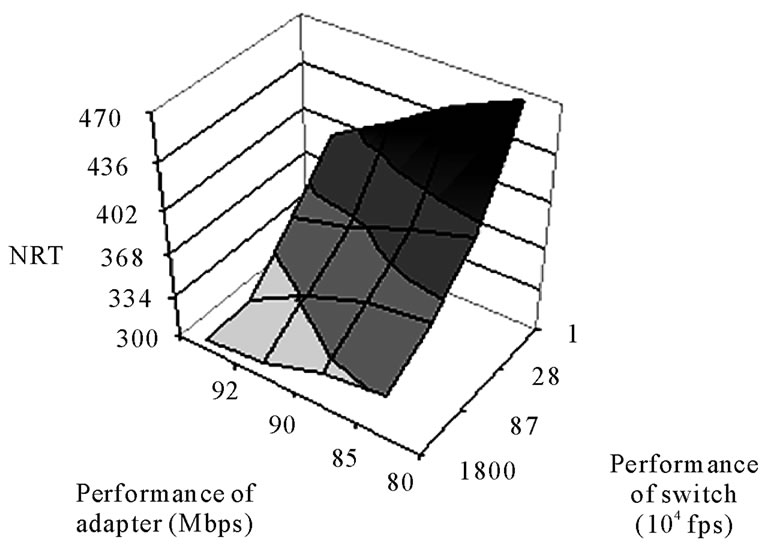 (c)
(c)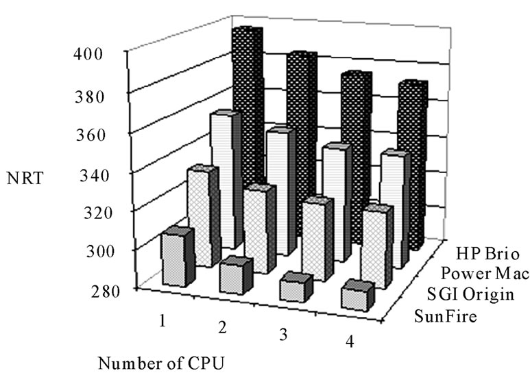 (d)
(d)
Figure 7. Variation of the network response time (NRT). (a) On performance of switches; (b) On size of buffer; (c) On network’s hardware; (d) On server’s hardware.
servers and switches. The model has a fixed number of nodes for an arbitrary given network and, moreover, it implements the evaluation of network response time as the major parameter of network’s performance.
As the structure of a given network is a parameter represented by the marking of dedicated places, it provides an easy reuse of the model which could be embedded into networks’ CAD systems.
The performance evaluation for the network of the railway dispatcher center was implemented. The obtained results may be used at the development of realtime systems.
8. References
[1] X. Zhang and G. F. Riley, “Bluetooth Simulations for Wireless Sensor Networks Using GTNetS,” Proceedings of 12th Annual Meeting of the IEEE/ACM International Symposium on Modeling, Analysis, and Simulation of Computer and Telecommunication Systems, Volendam, 5-7 October 2004, pp. 375-382.
[2] K. Jensen, “Colored Petri Nets—Basic Concepts, Analysis Methods and Practical Use,” Springer-Verlag, Berlin, Vol. 1-3, 1997.
[3] M. Beaudouin-Lafon, W. E. Mackay, M. Jensen, et al., “CPN Tools: A Tool for Editing and Simulating Coloured Petri Nets,” LNCS 2031: Tools and Algorithms for the Construction and Analysis of Systems, 2001, pp. 574-580. http://www.daimi.au.dk/CPNTools
[4] D. A. Zaitsev, “Verification of Protocol TCP via Decomposition of Petri Net Model into Functional Subnets,” Proceedings of the Poster Session of 12th Annual Meeting of the IEEE/ACM International Symposium on Modeling, Analysis, and Simulation of Computer and Telecommunication Systems, Volendam, 5-7 October 2004, pp. 73-75.
[5] D. A. Zaitsev, “An Evaluation of Network Response Time Using a Coloured Petri Net Model of Switched LAN,” 5th Workshop and Tutorial on Practical Use of Coloured Petri Nets and the CPN Tools, Aarhus, 8-11 October 2004, pp. 157-167.
[6] D. A. Zaitsev, “Switched LAN Simulation by Colored Petri Nets,” Mathematics and Computers in Simulation, vol. 65, no. 3, 2004, pp. 245-249. doi:10.1016/j.matcom. 2003.12.004
[7] D. A. Zaitsev and T. R. Shmeleva, “Modeling of Switched Local Area Networks by Colored Petri Nets,” Zviazok (Communications), vol. 46, no. 2, 2004, pp. 56-60.
[8] H. S. Zyabirov, G. A. Kuznetsov, F. A. Shevelev, et al., “Automated System for Operative Control of Exploitation Work GID Ural-VNIIZT,” Railway Transport, no. 2, 2003, pp. 36-45.
[9] R. Breyer and S. Riley, “Switched, Fast, and Gigabit Ethernet,” MacMillan Technical Publications, Indianapolis, 1999, pp. 1-618.
[10] S. Pahomov and S. Samohin, “Testing Fast Ethernet Adapters,” ComputerPress, no. 8, 2001.