Journal of Intelligent Learning Systems and Applications
Vol.4 No.3(2012), Article ID:22032,7 pages DOI:10.4236/jilsa.2012.43023
Systematic vs. Non-Systematic Search for 3D Aircraft Conflict Resolution
![]()
LIMIARF/FSR, University Mohammed V Agdal, Rabat, Morocco.
Email: ymechqrane@gmail.com, bouyakhf@fsr.ac.ma
Received November 22nd, 2011; revised March 31st, 2012; accepted April 7th, 2012
Keywords: Constraint Satisfaction Problem; Systematic Search; Non-Systematic Search; Aircraft Conflict Resolution
ABSTRACT
A conflict is an event in which two or more aircraft experience a loss of minimum separation. In this paper, we formulate the problem of solving conflicts arising among several aircraft moving in a shared airspace as a Constraint Satisfaction Problem (CSP). The constraint satisfaction problem being NP-complete, the algorithms developed to solve it have been of two types: non-systematic and systematic search methods. In this paper, we have considered a breakout algorithm as an example of non-systematic search methods and a backtracking procedure that maintains Arc Consistency (MAC) as an example of systematic search methods. The performance of these algorithms was compared experimentally and the Breakout algorithm is shown to be clearly superior.
1. Introduction
The annual cost to the airline industry due to the ATC caused delays is estimated to be $5.5 billion [1]. It is believed that by increasing the level of automation, the tasks of air traffic controllers can be simplified and the efficiency of flow of aircraft can be improved [2]. Recently, interest has grown toward developing advanced conflict detection and resolution systems to warn air traffic controllers and/or pilots about an imminent loss of separation between aircraft, and to assist them in their resolution. Conflict detection and resolution is performed at three different levels of the ATM process. 1) Long Range: Some form of conflict prediction and resolution is carried out over a time horizon of several hours. It involves composing flight plans and airline schedules (on a daily basis, for example) to ensure that airport and sector capacities are not exceeded; 2) Mid-Range: Conflict prediction and resolution is carried out by Air Traffic Controllers, over horizons of the order of tens of minutes. It involves modifying the flight plan on-line to ensure adequate aircraft separation; 3) Short Range: Conflict prediction and resolution is also carried out on board the aircraft, over horizons of seconds to minutes. The traffic alert and collision avoidance system, currently operating on all commercial aircraft carrying more than 30 passengers, is such a prediction/resolution algorithm.
In this paper, we focus on the mid-term conflict resolution problem which is an on-line problem. This problem can be stated as follows: Knowing the positions of aircraft at any given time and their future positions (to a fixed degree of accuracy) over the next ten minutes, what manoeuvring instructions should the Air Traffic Controller give to these aircraft so that the separation constraints are satisfied? A separation constraint is a relation between each pair of aircraft in the controlled airspace. This relation specifies that there exists a minimum distance that should be maintained at all times between the aircraft involved in this relation. The problem of conflict resolution is closely related to some problems in motion planning in the presence of moving obstacles. In general, these problems are known to be NP-hard [3]. This fact explains the large variety of existing conflict resolution algorithms. Already in 2000, Kuchar and Yang [4] listed over than 60 different approaches found in the literature. A more recent survey can be found in [5]. The studies of conflict resolution may be categorized into three different cases according to the methods by which a solution is obtained.
A first class of conflict resolution problem methods may be referred to as rule-based conflict resolution, in which a maneuver is resolved according to pre-described rules ([6-8] for example). Rule-based approaches might work for the case involving two aircraft, but may require a prohibitive number of rules to handle all situations arising when more than two aircraft are involved.
A second class of conflict resolution techniques uses force field methods and assumes that aircraft fly in the force field generated by a potential function; the forces induced by the potential function form a resolution maneuver (for example [9]). Although widely used for the motion control of mobile robots, force field methods have not yet been very popular in aircraft conflict resolution. This is due to the fact that these methods may produce maneuvers which real aircraft are incapable of performing.
A third class includes optimized conflict resolution. These methods produce a resolution maneuver which minimizes a given cost, a function of deviation from the original trajectory, flight time, fuel consumption, or energy. Contributions belonging to this category include, but are not limited to [10-15]. However, these methods usually need to make one or more unrealistic assumptions when extrapolating the future positions of aircraft (for example, no uncertainty about the aircraft speed).
In this paper, we propose a Constraint Programming based conflict resolution approach for ensuring adequate aircraft separation in air traffic control systems. We present a CSP model where the separation constraints are expressed in a declarative form that allows taking into account speed uncertainties. The constraint satisfaction problem being NP-complete, the algorithms developed to solve it have been of two types: non-systematic and systematic search methods. Generally, non-systematic search methods alter incrementally inconsistent value assignments to all the variables. They use a repair or hill climbing metaphor to move towards more and more complete solutions. To avoid getting stuck at local minimum they are equipped with various devices for randomising the search. Systematic search methods are often based on a depth-first search algorithm with backtracking where at each step of the search, a variable assignment is performed followed by a process called constraint propagation. In this paper, the problem is tackled with two of the best known systematic and local search algorithms. The systematic search is a chronological backtracking equipped with a filtering algorithm that maintains arc consistency (MAC) and the local search is a Breakout algorithm (BO).
The remainder of this paper is organized as follows: Some basic definitions are recalled in Section 2; Afterwards, the problem is formulated as a constraint satisfaction problem in Section 3; Then, the conflict resolution algorithms are introduced in Section 4; Simulation results are given in Section 5 before the conclusion of the paper in Section 6.
2. Preliminaries
Constraint Satisfaction Problems (CSPs) occur widely in artificial intelligence. They involve finding values for problem variables subject to constraints which restrict acceptable combinations.
Definition:
A Constraint Network is defined by:
1) a finite set of variables X = {x1, ···, xn}.
2) a domain for X, that is, a set D(x1) × ···× D(xn), where D(xi) denotes the set of values allowed for xi.
3) a finite set C = {c1, ···, ce} of constraints. A constraint c involves the variables in the set var s(c) and specifies the allowed tuples (i.e. combinations) of these variables.
A solution to a constraint network is an assignment of values to all the variables such that all the constraints are satisfied. A constraint network is said to be satisfiable if it admits at least a solution. The Constraint Satisfaction Problem (CSP) is to determine whether or not a given constraint network, also called CSP instance, is satisfiable.
3. Formulating the Conflict Resolution Problem as a CSP
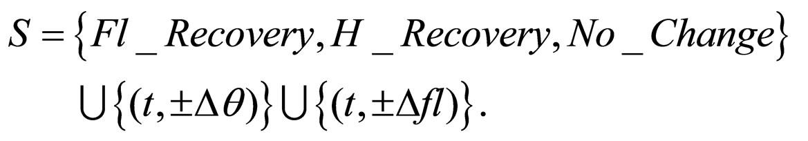
We consider n aircraft flying in the same region of the airspace, each following its individual flight plan. The flight plan is assumed to consist of a sequence of flight levels, a sequence of way points and a sequence of speeds for moving between them. A conflict is an event in which two or more aircraft come closer than a safety distance to one another. The safety distance is encoded by means of a minimum allowed horizontal separation (i.e. D) and a minimum vertical separation (i.e. H). One example criterion is D = 5 nautical miles and H = 1000 ft. These values correspond to the current en-route separation standard at lower altitudes. In this paper, to avoid a conflict, an aircraft may perform a heading change (t, ±Δθ) or a flight level change (t, ±Δfl), where t is the time when the aircraft starts its maneuver. In addition to heading and flight level changes, we also define some special maneuvers: 1) The maneuver No_change means that the aircraft will still in its current path without performing any change; 2) If an aircraft is currently flying in a flight level different than its nominal (i.e. desired) flight level, the maneuver Fl_Recovery brings back this aircraft to its nominal flight level; 3) The maneuver H_Recovery directs an aircraft at the next way point in its flight plan. The conflict detection and resolution functions are executed periodically, corresponding to the update cycle (1 minute in our numerical experiments). Hence, the maneuvers Fl_Recovery and H_Recovery will allow aircraft that were deviated from their initial paths during the previous cycles to return to their nominal trajectories. That is, the set of potential maneuvers for each aircraft is
During each cycle, each aircraft may make a single maneuver to return to its preferred path or to avoid a conflict. The idea is to find a solution which removes all possible collisions.
We assume that there is an error about the aircraft’s future location because of ground speed prediction uncertainties. The uncertainties on climbing and descending rates are even more important. As the conflict free trajectory must be robust regarding these and many other uncertainties, an aircraft is represented by a point at the initial time. But the point becomes a line segment in the uncertainty direction (the speed direction here, see Figure 1). The first point of the line “flies” at the maximum possible speed, and the last point at the minimum possible speed. When changing direction (t = 4), the segment becomes a parallelogram that increases in the speed direction. To check if two aircraft are in conflict, we compute at each time step of the simulation the distance between the two polygons modelling the future aircraft positions and compare it to the standard separation. In the vertical plane, we use a cylindrical modelling (Figure 1). Each aircraft has a mean altitude, a maximal altitude and a minimal altitude. To check if two aircraft are in conflict, the minimal altitude of the higher aircraft is compared to the maximal altitude of the lower aircraft.
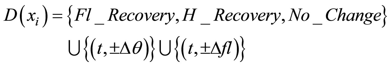
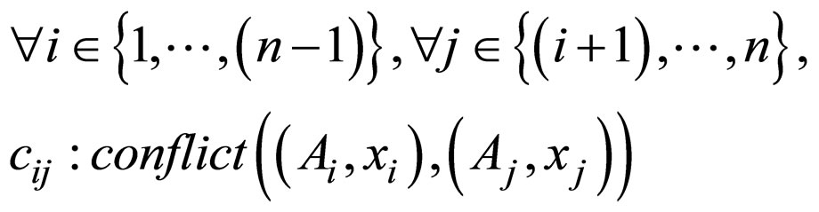
That is, let a and b be two possible maneuvers for two aircraft Ai and Aj. Let traj(Ai, a) be the modified trajectory of the aircraft Ai if it executes the maneuver a. The boolean function conflict((Ai, a), traj(Aj, b)) returns true if traj(Ai, a) and traj(Aj, b) will generate a conflict. We can now state our CSP model as follows. Let n be the number of aircraft in the controlled air space. We associate with each aircraft Ai a variable xi which takes its values in
We have the following constraints:
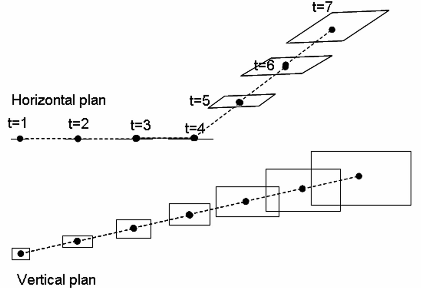
Figure 1. Modelling of speed uncertainties.
4. The Conflict Resolution Algorithms
As already mentioned, there is two types of algorithms developed to solve the CSPs: non-systematic and systematic search methods. In this paper, we have considered a breakout algorithm as an example of non-systematic search methods and a backtracking procedure that maintains Arc Consistency as an example of systematic search.
4.1. The Breakout Algorithm
The breakout algorithm [16,17] is given in Algorithm 1. In this algorithm, the sate 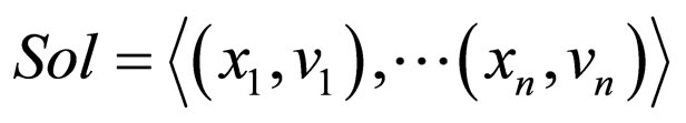 is a flawed solution that may contains some constraint violations, where vi or Sol(xi) denote the value assigned to xi in Sol. The breakout algorithm contains two essential steps: determining the local change that minimizes conflicts, and increasing the weights (called the breakout). We associate with every constraint c a weight wt(c). All weights are positive integer numbers and are set to 1 initially. Conflict minimization consists of choosing a variable xi and a new value vi
  D(xi) such that the conflicts in the current state are reduced as much as possible. To this end, we compute for every variable its conflict value, defined as follows:
Definition
The conflict value WT(xi, vi’) of a variable xi assigned the value vi in Sol is the sum of weights of the constraints involving xi that would be violated in a state Sol’ that differs from Sol only in that xi is assigned vi’.
The best improvement is to the variable/value combination xi, vi such that WT(xi, Sol(xi)) – WT(xi, vi’) is largest. If there is such a combination with an improvement greater than 0, the variable/value combination with the best improvement is chosen as the local improvement. If no improvement is possible by changing the value of any variable, the current state is called a local minimum.
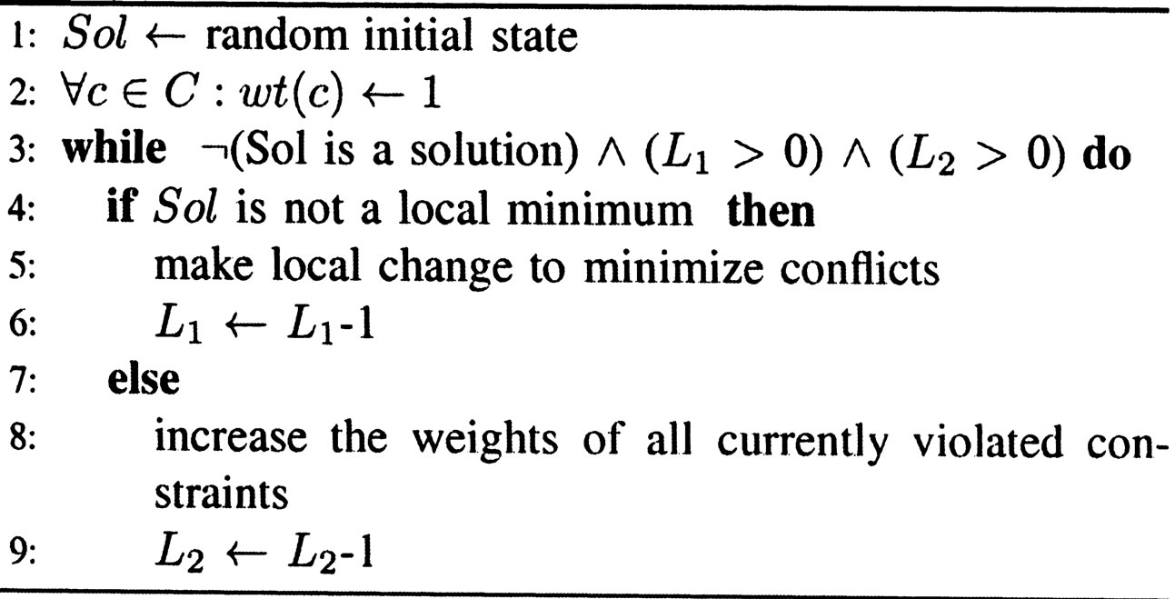
Algorithm 1. The breakout algorithm.
When trapped in a local-minimum, the breakout algorithm increases the weights of violated constraint in the current state by 1 so that the evaluation value of the current state becomes larger than the neighbouring states; thus the algorithm can escape from a local-minimum. Increasing the weights of violated constraint is what is called a breakout step. In general, one imposes a runtime limit on the algorithm: there is a limit on the number of iterations denoted by L1, i.e. the number of times variables are revised, and on the number of breakout steps denoted by L2.
4.2. The Backtracking Algorithm
The most common algorithm for performing systematic search is backtracking. Backtracking incrementally attempts to extend a partial solution that specifies consistent values for some of the variables, toward a complete solution, by repeatedly assigning a value for another variable consistent with the values in the current partial solution. A dead-end occurs when all the values of the current variable (i.e. the variable being instantiated) are rejected. In such a case, the variable that was instantiated before the current variable becomes uninstantiated. This process is called backtracking. The backtracking algorithm terminates when all possible assignments have been tested or a solution have been found. Usually, each variable assignment is followed by a process that consists in inferring some infeasible values (i.e. filtering). Arc consistency is the oldest way of propagating constraints. Arc consistency can be defined for binary constraints (i.e. constraints involving two variables) as follows:
Definition
Given a network N = (X, D, C), a binary constraint c  C such that var s(c) = {x, y}. A value a
  D(x) is consistent with c if there exists a value b
  D(y) such that (a, b) satisfies c. The value b is called a support for x on c. A variable x is arc consistent on the constraint c if all values in D(x) are consistent with c. The constraint c is arc consistent if x and y are arc consistent on c.
The most well-known algorithm for arc consistency is AC3 [18]. It was proposed for binary networks and actually achieves arc consistency.
Function mac(X, D, C) of Algorithm 2 is a backtracking algorithm that follows an AC3 like schema of propagation. This function maintains a list Q of all the pairs (x, c) for which we are not guaranteed that D(x) is arc consistent on c. In line 1, Q is initialized with all possible pairs (x, c) such that c  C and x
  var s(c). Afterwards, the function propagare() is called (line 2). The main loop (line 24) of the function propagare() picks the pairs (x, c) in Q one by one and calls revise(x, c) (line 26) to ensure that every remaining value in D(x) has a support
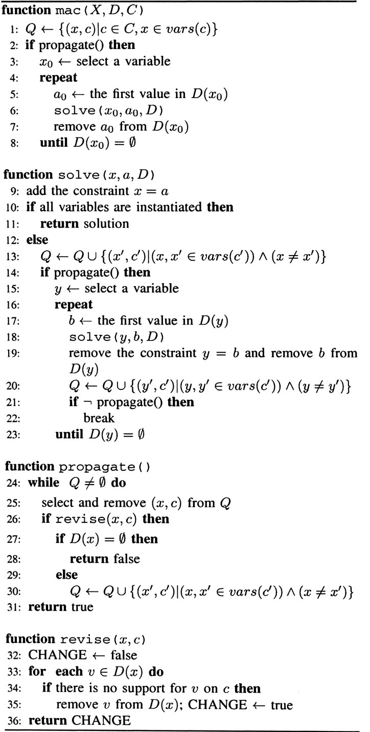
on c. During the execution of the function propagare(), each time a domain D(x) is modified (line 26), it can be the case that a value for another variable x’ has lost its support on a constraint c’ involving both x and x’. Hence, all pairs (x, c’) such that x, x’  var s(c’) must be put again in Q (line 30).
When Q is empty, the function propagare() returns true (line 31) as we are guaranteed that all remaining values of all variables are consistent with all constraints. When a domain D(x) is wiped out (line 27), the function propagare() returns false (line 28).
If the initial call of the function propagare() was successful (line 2), the function mac() selects a variable x0 and the first value a0 in D(x0) and calls the recursive function solve(x0, a0, D). If no solution can be found with x0 = a0 this value is definitely removed from D(x0) (line 7) and the next value for is attempted. The problem has no solution if all the values in D(x0) are impossible. The recursive function solve(x, a, D) takes as arguments a variable x, a value a  D(x) and D, i.e. the current domains of the variables D = D(x1) × ··· ×D(xn), where D(xi) denotes the current domain of xi. First, the function solve(x0, a0, D) assigns the value a to the variable x (i.e. D(x) is reduced to a single value {a} by adding the constraint x = a). Afterwards, if all the variables are instantiated then a solution is found, otherwise, since the domain of x was modified, the function propagare() is called in order to maintain the arc consistency. If the call of the propagation mechanism was successful (line 14), a new variable y and a new value b in D(y) are selected and a recursive call to the function solve(y, b, D) is made. If a backtracking occurs (line 19), the variable y is uninstantiated by removing the constraint y =b, and the value b is removed from the current domain of y. This removal is once again propagated (line 20).
The order in which variables are assigned by a backtracking search algorithm has been recognized as a key issue for a long time. In this paper we used the domain size over the weighted degree heuristic (i.e. dom/wdeg) introduced in [19]. This heuristic guides the search toward hard parts of a CSP by first instantiating variables involved in the constraints that have frequently participated in dead-end situations.
5. Experimental Results
In our experiments, all aircraft fly at the same velocity, 500 miles per hour. Aircraft must maintain a minimum horizontal separation distance D = 5 nautical miles, and a minimum vertical separation distance H = 1000 ft. The prediction is done for a lookahead window of length T = 10 min. Time is discretized and the timestep is 15 s. The set of possible heading changes is Δθ = ±30, ±20, ±10. Aircraft are flying on three distinct flight levels (i.e., 350, 360, 370) but can change levels to avoid conflicts.
Our conflict resolution algorithms were coded using java. The computational times were computed on an Intel P4 machine with 1 G RAM under Linux (Ubnutu 6.06).
5.1. 2D-Scenarios
At first, to compare the performance of algorithms in terms of computational time, changes in altitude are not allowed; this enriches the problem by requiring fewer aircraft to create a dense airspace. In the first group of simulations, we consider that a predetermined number of aircraft are randomly distributed inside a circle with a radius of 70 miles and each aircraft is assigned a random heading. Aircraft are generated so that they are not involved in a conflict immediately (all conflicts occur after one minute). We vary the number n of generated aircraft from 5 to 30 aircraft by steps of 5. For each value of n we generated 25 different instances. In Table 1 we show the averaged computational times (in seconds) for each algorithm.
In the second group of simulations, we generated symmetric scenarios where a predetermined number of aircraft are evenly distributed on a circle with a radius of 70 miles (Figure 2). These scenarios are similar to those considered by many other researchers ([13] for example).
The destination for these aircraft is the exact opposite side of the circle from their originating position. This means that in the absence of maneuvers all aircraft would conflict at the origin of the circle. We vary the number n of generated aircraft from 5 to 40 aircraft by steps of 5. In Table 2 we indicate the computational times (in seconds) needed by each algorithm to find the solution.
Those results show that BO is not only faster than MAC, but also that BO is able to solve problems much larger than MAC. The poor performance of the systematic search method is likely the result of its inability to quickly revise a bad decision. Indeed, in systematic methods, the partial solution constructed during the search process will not be revised unless it is proven that there exists no complete solution subsuming the partial solution. If the algorithm makes a bad selection of a variable value, the algorithm must perform an exhaustive search for the partial solution in order to revise the bad decision. When the problem becomes very large, doing such an exhaustive search is very expensive.
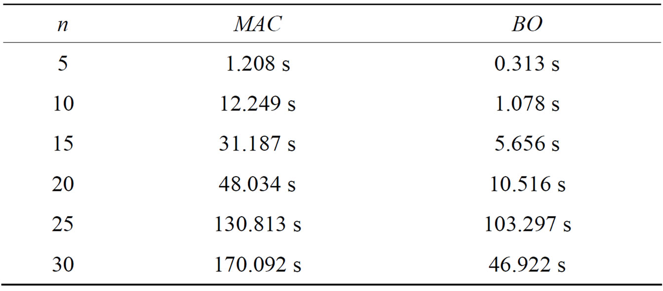
Table 1. Computational times for random scenarios.
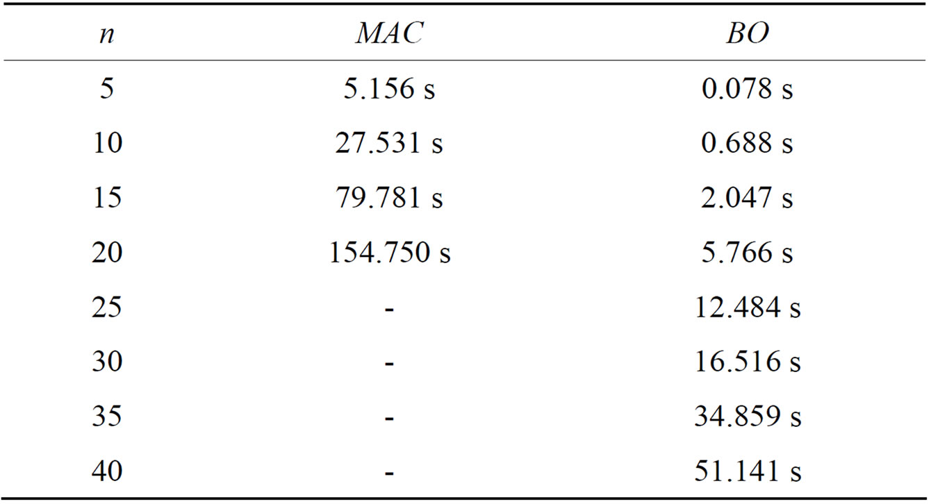
Table 2. Computational times for symetric scenarios.
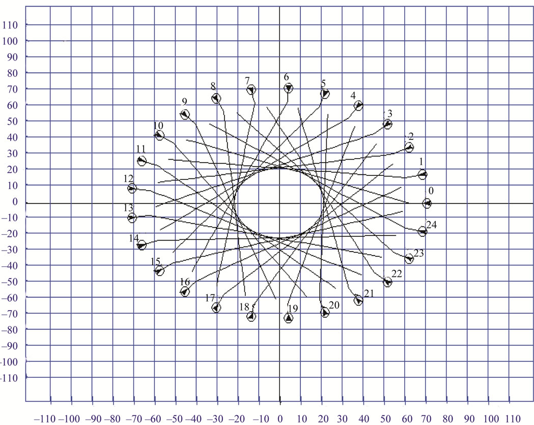
Figure 2. A symmetric scenario of 25 aircraft. The trajectories that must follow the aircraft to avoid conflicts are plotted.
5.2. 3D-Scenarios
The systematic and non-systematic search methods have different strategies for choosing values and variables. In the following, we seek to examine the consequences of these differences on the behaviour of algorithms. To this end, a 3-dimensional airspace, with 3 flight levels was simulated. The airspace is a 200 nautical miles sided square. 60 aircraft are flying on three distinct flight levels and can change levels to avoid conflicts. Aircraft are flying Westbound on the first and the third flight levels and Eastbound on the second flight level.
Aircraft that leave the controlled airspace are replaced. We considered a scenario lasting Tsim = 50 min instead of snap shot scenarios considered in the first group of the simulations. Over the course of the full simulation time, a look-ahead window of length T = 10 min is advanced in 1-minutes steps, corresponding to the conflict resolution update cycle. Hence, conflict resolution is performed over a series of 10-minute time windows, corresponding to the intervals [0, 10], [1, 11], ···, [ti, ti + 10], ···, [Tsim – 10, Tsim] over the duration of the simulation. Initially, aircraft are generated so that they are not immediately involved in a conflict (i.e. there is no conflict between aircraft during the interval [0, 1]). At each time ti, we perform conflict resolution for the interval [(ti + 1), (ti + 1) + 10]. We then modify the routes accordingly, advance the 10- minute window by 1 minute and continue. New aircraft are generated so that they are not immediately involved in a conflict with the aircraft that are still in the sector (i.e. all conflicts with the aircraft that are still in the sector occur after 1 min). In Table 3, we indicate by #conflicts the number of total conflicts solved over the duration of the simulation and by #hor. (respectively #ver.), the number of horizontal (respectively vertical) maneuvers executed over the duration of the simulation.
We notice that MAC tends to resolve conflicts in the horizontal plan (the number of horizontal maneuvers is higher for MAC) while BO makes a frequent use of vertical maneuvers (the number of vertical maneuvers is higher for BO). The conflict resolution in the horizontal plan would be more likely to create new conflicts with neighboring aircraft during subsequent conflict resolutions. This may explain why the total number of resolved conflicts is higher for MAC.
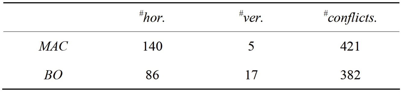
Table 3. 3D scenarios.
6. Conclusion
In this paper, the aircraft conflict resolution problem was formulated as a constraint satisfaction problem. Afterwards, a systematic search method and a non-systematic search method were put in competition. The performance of these methods was compared using a variety of scenarios and the non-systematic search method was shown to be more effective in resolving conflicts.
REFERENCES
- T. S. Perry, “In Search of the Future of Air Traffic Control,” IEEE Spectrum, Vol. 34, No. 8, 1997, pp. 18-35. doi:10.1109/6.609472
- Joint Planning and Development Office, “Next Generation Air Transportation System Integrated Plan,” Washington DC, 2004.
- J. H. Reif and M. Sharir, “Motion Planning in the Presence of Moving Obstacles,” 25th IEEE Symposium on Foundations of Computer Science, Portland, 21-23 October 1985, pp. 144-154,
- J. Kuchar and L. C. Yang, “A Review of Conflict Detection and Resolution Modeling Methods,” IEEE Transactions on Intelligent Transportation Systems, Vol. 1, No. 4, 2000, pp. 179-189.
- G. Chaloulos, J. Lygeros, I. Roussos, K. Kyriakopoulos, E. Siva, A. Lecchini-Visintini and P. Casek, “Comparative Study of Conflict Resolution Methods,”, iFly Project, 2009.
- K. Bilimoria, B. Sridhar and G. Chatterji, “Effects of Conflict Resolution Maneuvers and Traffic Density of Free Flight,” AIAA Guidance, Navigation, and Control Conference, San Diego, 29-31 July 1996.
- B. Carpenter and J. Kuchar, “Probability-Based Collision Alerting Logic for Closely-Spaced Parallel Approach,” Proceedings of the AIAA 35th Aerospace Sciences Meeting and Exhibit, Reno NV, 6-9 January 1997.
- V. Duong, E. Hoffman, L. Floc’hic and J. P. Nicolaon, “Extended Flight Rules to Apply to the Resolution of Encounters in Autonomous Airborne Separation,” Technical Report, EUROCONTROL Experimental Center 1996.
- K. Zeghal, “A Review of Different Approaches Based on Force Fields for Airborne Conflict Resolution,” AIAA Guidance, Navigation, and Control Conference, Boston, 10-12 August 1998, pp. 818-827.
- E. Frazzoli, Z. H. Mao, J. H. Oh and E. Feron, “Aircraft Conflict Resolution via Semi-definite Programming,” AIAA Journal of Guidance, Control, and Dynamics, Vol. 24, No. 1, 2001, pp. 79-86. doi:10.2514/2.4678
- J. Hu, M. Prandini and S. Sastry, “Optimal Coordinated Maneuvers for Three Dimensional Aircraft Conflict Resolution,” AIAA Journal of Guidance, Control and Dynamics, Vol. 25, No. 5, 2002, pp. 888-900. doi:10.2514/2.4982
- A. U. Raghunathan, V. Gopal, D. Subramanian, L. T. Biegler and T. Samad, “Dynamic Optimization Strategies for Three-Dimensional Conflict Resolution of Multiple Aircraft,” Journal of Guidance, Control, and Dynamics, Vol. 27, No. 4, 2004, pp. 586-594. doi:10.2514/1.11168
- L. Pallottino, E. Feron and A. Bicchi, “Conflict Resolution Problems for Air Traffic Management Systems Solved with Mixed Integer Programming,” IEEE Transactions on Intelligent Transportation Systems, Vol. 3, No. 1, 2002, pp. 3-11. doi:10.1109/6979.994791
- G. Gariel and E. Feron, “3D Conflict Avoidance under Uncertainties,” 28th Digital Avionics Systems Conference, Orlando, 23-29 October 2009, pp. 4.E.3-1-4.E.3-8.
- E. M. Kan1, M. H. Lim, S. P. Yeo, J. S. Ho and Z. Shao, “Contour Based Path Planning with B-Spline Trajectory Generation for Unmanned Aerial Vehicles (UAVs) over Hostile Terrain,” Journal of Intelligent Learning Systems and Applications, Vol. 3, No. 3, 2011, pp. 122-130.
- S. Minton, M. Johnston, A. Philips and P. Laird, “Minimizing Conflicts, A Heuristic Repair Method for Constraint Satisfaction and Scheduling Problems,” Artificial Intelligence, Vol. 58, No. 1-3, 1992, pp. 161-205. doi:10.1016/0004-3702(92)90007-K
- P. Morris, “The Breakout Method for Escaping from Local Minima,” 11th National Conference on Artificial Intelligence, Washington DC, 11-15 July 1993, p. 4045.
- A. K. Mackworth, “Consistency in Networks of Relations,” Artificial Intelligence, Vol. 8, No. 1, 1977, pp. 99- 118. doi:10.1016/0004-3702(77)90007-8
- F. Boussemart, F. Hemery, C. Lecoutre and L. Sais, “Boosting Systematic Search by Weighting Constraints,” Proceedings of ECAI’04, Valencia, 22-27 August 2004, pp. 146-150.