Journal of Water Resource and Protection
Vol.4 No.9(2012), Article ID:22470,9 pages DOI:10.4236/jwarp.2012.49087
Comparison of Potential Bio-Energy Feedstock Production and Water Quality Impacts Using a Modeling Approach
Department of Agricultural and Biological Engineering, Mississippi State University, Starkville, USA
Email: pparajuli@abe.msstate.edu
Received July 27, 2012; revised August 24, 2012; accepted August 30, 2012
Keywords: Biofuels; Feedstock Yield; Stream Flow; Water Quality; SWAT; Watershed
ABSTRACT
Cellulosic and agricultural bio-energy crops can be utilized as feedstock source for bio-fuels production and provide environmental benefits such as hydrology, water quality. This study compared potential feedstock yield and water quality benefit scenarios of six bio-energy crops: Miscanthus (Miscanthus-giganteus), Switchgrass (Panicum virgatum), Johnsongrass (Sorghum halepense), Alfalfa (Medicago sativa L.), Corn (Zea mays), and Soybean {Glycine max (L.) Merr.} at the watershed scale using Soil and Water Assessment Tool (SWAT) model. The SWAT model was calibrated (1998 to 2002) and validated (2003 to 2010) using monthly measured USGS stream flow data. Model was further verified using available monthly sediment yield, and county level NASS corn and soybean yield data within the watershed. The long-term average annual potential feedstock yield as an alternative energy source was determined the greatest when growing Miscanthus grass scenario (21.9 Mg/ha) followed by Switchgrass (15.2 Mg/ha), Johnsongrass (12.1 Mg/ha), Alfalfa (7 Mg/ha), Corn (5.9 Mg/ha), and Soybean (2.35 Mg/ha). Model results determined the least amount of average annual sediment yield (1.1 Mg/ha) from the Miscanthus grass scenario and the greatest amount (12 Mg/ha) from the corn crop scenario. About 11% less annual average surface water flow from the watershed could be anticipated when converting land areas from soybean to Miscanthus grass. The results of this study suggested that growing Miscanthus grass in the UPRW would have the greatest potential feedstock yield and water quality benefits. The results of this study may help in developing future watershed management programs.
1. Introduction
The world’s energy consumption will be increased by 54% from 2001 to 2025, which impacts on CO2 increase by 55% for the same period [1]. Although, US CO2 emission in 2009 is reported slightly decreased due to economic impact on energy use [2]; it is estimated to rise significantly until 2025 [3] due to increase in the population from 6.9 billion in 2011 to 9.4 billion in 2050 and 10.4 billion by 2100 [4]. Increased CO2 emission impacts and bio-fuels needs could be benefitted with promoting cellulosic feedstock sources such as Switchgrass in the locally available agricultural marginal lands [5,6]. Growing bio-fuels demand in view of water quality and energy impact related with biofuels production need additional research.
Several study in the past [5,7,8] reported benefits and limitations of food-based and non-food-based feedstock sources in terms of their energy, CO2, and bio-fuel productions. Increasing level of research is needed on cellulosic bio-energy crop sources as they can be an alternative feedstock sources to produce bio-fuels. The production of various feedstock sources could have different levels of environmental impacts (e.g. water quality, potential bio-energy) as each feedstock sources are managed differently in the agricultural landscapes. In addition to several traditionally growing potential bio-energy feedstock sources (e.g. Johnsongrass, Alfalfa, Corn, Soybean), Miscanthus and Switchgrass are being considered as a promising crops for environment and feedstock sources. The Miscanthus or Giant Miscanthus or (Miscanthus × giganteus) feedstock source is characterized as a perennial grass, which is a very tall grass, and grows very well during warm-season of the year. Miscanthus is considered as one of the main feedstock source for the bio-fuel industries and it is under experimental research [9]. Miscanthus has been evaluated in the Mississippi State University over the past 5 - 10 years as an alternative grass for the biofuels. Since the plant can get as tall as 4 m, it can yield up to 50 Mg per ha per year in Mississippi [10].
The Switchgrass was recognized as one of the best bio-energy crops for further study as it was successfully tested by some universities in the various geographic regions (e.g. Auburn University, AL; Virginia Tech., VA;
Purdue University, IN; Iowa State University, IA) of the country [11]. The Switchgrass was determined as a suitable alternative bio-energy crop due to several benefits including high yielding crop, capable to grow on minor agricultural lands, and low management input costs. The Switchgrass is an alternative to the corn crop due to greater energy productivity [12]. Cultivation of Switchgrass can help in reducing more soil erosion and nutrients as compare to the traditional crops [13]. It is estimated that Switchgrass can produce about 260.8 GJ per ha of average energy at a production level of approximately 25 Mg per ha per year [10] in the southeast US.
Sedimentation, biological impairments, pathogens, organic enrichment and nutrients are considered five major causes of water body contamination in the state of Mississippi [14]. The Ross Barnett Reservoir (RBR) receives waters from the UPRW (Figure 1) and it is considered as one of the important surface water bodies in the state of Mississippi that has been utilized for supplying daily drinking water to the people of Jackson and its surrounding areas in Mississippi, and recreational use for the significant number of visitors every year. Although various field level studies have been carried out in the past to assess biomass and feedstock yields of several bio-energy crops, the study of their effects on environment and water quality is still limited. An evaluation of the bio-energy crop yield potential response to the water quality benefits is essential for the watershed that drains into the RBR. The plant growth models such as ErosionProductivity Impact Calculator (EPIC) [15] in conjunction with hydrologic simulation tools such as the SWAT [16] model can be used to investigate potential crop yields, water quality and hydrologic impacts (e.g. surface runoff, water yield, sediment yield, potential evapotranspiration) due to land use change.
A broad analysis of the articles published previously reported that the SWAT model is a useful model for evaluating the impact of agricultural practices on hydrology, crop yield, and water quality [17-20]. The SWAT watershed and water quality model application, calibration, and validation have been performed to assess surface runoff, sediment and nutrient yields, and bacteria loadings from several geographically referenced locations [17, 21]. The most of the previous modeling studies considered only hydrology and water resources implications. Previous literatures are limited in using SWAT model to evaluate the hydrologic and water quality benefits of changing land use area to bio-energy crops at watershed scale. The SWAT model was applied in the Delaware watershed (3000 km2) of northeast Kansas [22] to evaluate crop yield, water quality and economic benefits of bio-energy crop. However the authors evaluated only Switchgrass yield, it’s economic and water quality benefits. Previous studies [23,24] assessed performance of the
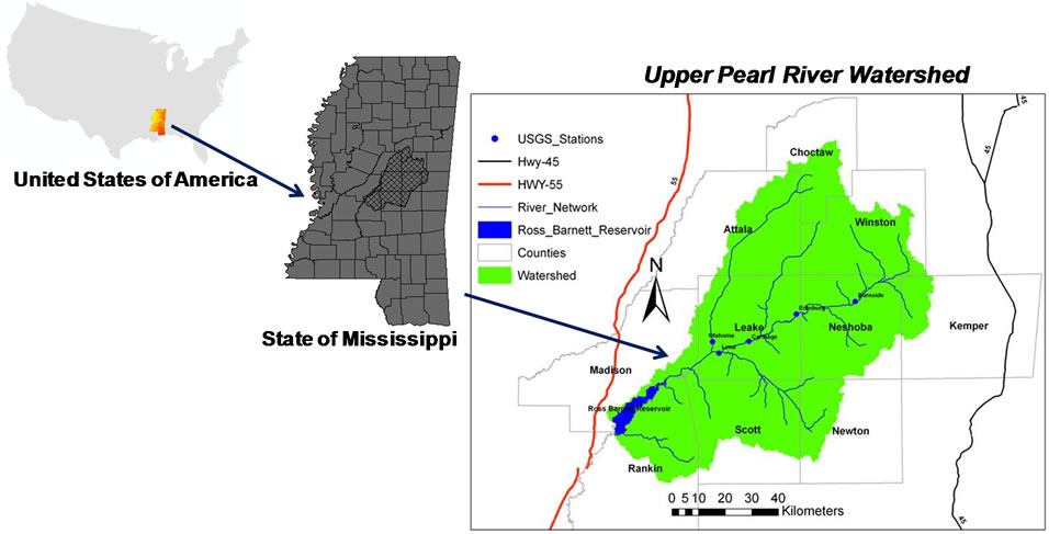
Figure 1. Study watershed: Upper Pearl River watershed in Mississippi.
SWAT and empirical geographic models respectively in the regional scales to predict Switchgrass yield. Authors did not evaluate feedstock yields of other bio-energy crops such as Miscanthus. Several studies investigated other conventional bio-energy crop yields separately such as corn and soybean [25]; Alfalfa [26]; and Johnsongrass [27]. It is yet to study hydrologic and water quality responses of bio-energy crops to adopt better water management practices. The objective of this study was to compare impact of bio-energy crop production on water quality at watershed scale using a modeling approach.
2. Materials and Methods
2.1. Watershed and Model
This modeling study was performed within the Upper Pearl River watershed (UPRW), which is located in the east-central, Mississippi. The UPRW encompasses 7588 km2 (Figure 1) area. The majority of the landuse in the watershed is covered by woodlands (72%) as followed by grassland (20%). The urban and other land use area covers about 8% of the watershed.
The SWAT model [16,28] is a physically based, continuous, daily time step model, which allowed predicting surface runoff, sediment and nutrient yields, pesticide, bacteria, and crop yields. The SWAT model sub-divides watershed into sub-basins and small spatial units called the hydrologic response units (HRUs). As the HRUs are generated based on the intersection of unique land use and soil conditions used in the model, spatially variable input parameters can be provided in the model. These input parameters can directly impact on the hydrology, water quality and crop yields. The SWAT model estimates daily time-period parameters (e.g. runoff, evapotranspiration), which is largely driven by daily rainfall inputs in the model. The variability in the crop growth functions are simulated in the SWAT model, which also utilizes the EPIC model. In the SWAT model all the available heat units above the base temperature helps crop-growth and crop-development. The SWAT model keeps the records of the daily sum of the heat units and daily average temperature must be greater than the base temperature for the crop growth [28].
The SWAT model needs several geospatial data inputs that cover the watershed boundary (e.g. Digital Elevation Model (DEM) grid data, land use, soil). The model uses these geospatial input parameters to develop specific model inputs for each HRU and sub-basins in the watershed. The 30 m × 30 m grid DEM data from the US Geological Survey [29] was used to create the UPRW watershed boundaries; State Soil Geographic Database (STATSGO) [30] was utilized to develop a soil input data for the entire watershed; and cropland data layer [31] was used to create model input land use data. Model also utilized daily measured rainfall and temperatures data as a climate data input from the ground based climate stations maintained by the National Climatic Data Center [32]. The Penman-Monteith potential evapotranspiration (PET) method used in this study requires daily rainfall, temperatures (both min. and max.), solar-radiation, relative-humidity, and wind-speed data input in model. Although, this study is benefited of using daily rainfall and temperatures data from the ground-based climate stations the other data required to use in the PET method in the model were not available from these climate stations. These unavailable data from the ground-based stations were generated by the SWAT model for the entire model simulation period [28].
2.2. Watershed Management and Bio-Energy Crops
Depending up on the land use data layer input in the model, the SWAT model estimated that out of 72% of the forest land use in the watershed evergreen, mixed, and deciduous forest trees cover about 22%, 20%, and 30% forest land use area respectively. At present, Bahiagrass is the dominant grass species in the 20% of grassland or pastureland of the UPRW (Curt Readus, NRCS, MS 2009, personal-communication) [21]. The warmseason crops are planted during April 15 and harvested during September 15 whereas cool-season crops are planted during October 15 and harvested during June 15. Conservation or minimum tillage is a management practice, which is commonly applied in the UPRW (Curt Readus, NRCS, MS, 2009, personal-communication) [21]. The production of the bio-energy crops (Miscanthus, Alamo Switchgrass, Johnsongrass, Alfalfa, Corn and Soybean), simulated in this study were evaluated on two land uses (croplands and pasturelands) and two soil groups (MS048 and MS089) that typically produce corn, soybean, and pasture crops. All the bio-energy crops were treated equally with auto irrigation based on plant water demand and auto fertilization method in the model [28]. This study compared potential feedstock yield of six bio-energy crops using the SWAT model. The SWAT model developed detail crop database for the Switchgrass (Alamo), Alfalfa, Johnsongrass, Corn and Soybean. There is no crop database developed for Miscanthus grass yet in the SWAT model. This study modified Miscanthus grass database from Switchgrass considering some important crop data as reported by literatures (Table 1) including maximum canopy height of 4.0 m [33,34] maximum leaf area index of 8.0 m2/m2 [35], and maximum root depths of 2.0 m [36].
2.3. Calibration, Validation and Analysis
The SWAT 2005 model was calibrated and validated changing one key parameter at a time manually similar to previous study [21] to evaluate hydrologic part of the model. The SWAT model predicted results were compared with the field measured data utilizing commonly used statistical parameters such as mean, correlation-coefficient (R2), and Nash-Sutcliffe efficiency (E) categories as recommended by previous literatures [19,37]. Author [21] classified the SWAT model performances of the monthly flow simulations using six categories (excellent if R2 and E ≥ 0.90; very good if R2 and E = 0.75 - 0.89; good if R2 and E = 0.50 - 0.74; fair if R2 and E = 0.25 - 0.49, and poor if R2 and E = 0 - 0.24; and unsatisfactory if R2 and E < 0).
3. Results and Discussion
The following sections (flow and sediment, bio-energy feedstock yields, and water quality) present results and discussion including model calibration, and validation.
3.1. Flow and Sediment
The assessment of the SWAT model in the UPRW for monthly stream-flow estimated good performances (R2 from 0.64 to 0.75 and E from 0.67 to 0.73) during model calibration at Lena and Edinburg gage stations (Figure 2(a) and Figure 3(a)). The SWAT model results for the stream flow simulation found slightly de-

Table 1. Comparative crop database parameters used in the SWAT model.
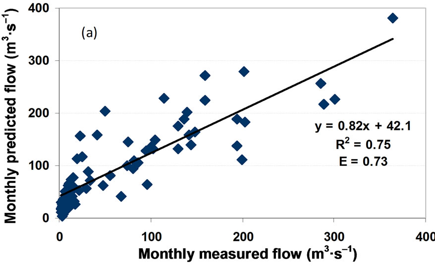
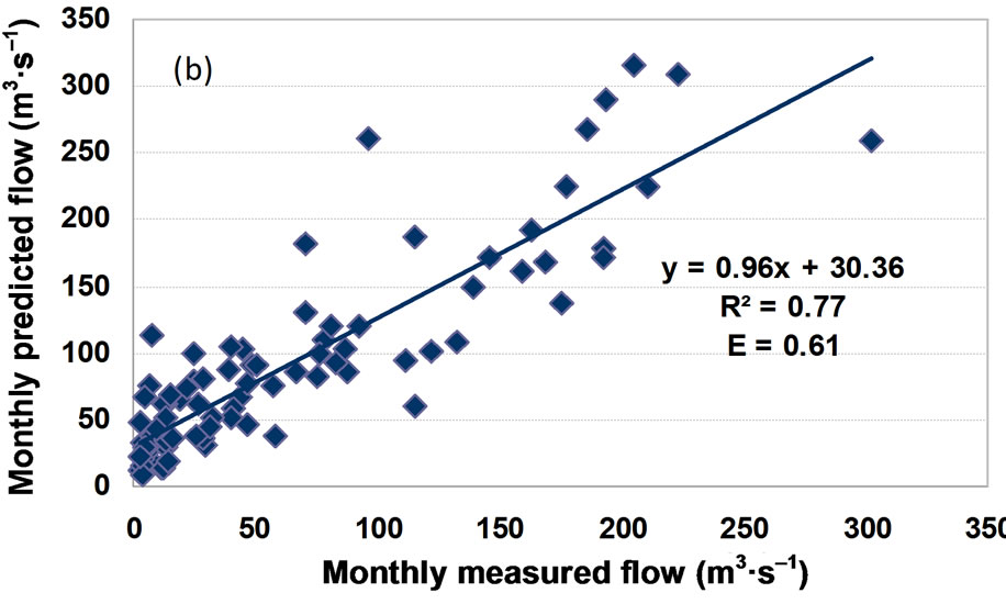
Figure 2. Model responses to monthly observed flow (m3/s) from the Lena USGS gage station in the watershed.


Figure 3. Model responses to monthly observed flow (m3/s) from the Edinburg USGS gage station in the watershed.
creased but good performance during model validation (R2 from 0.55 to 0.77 and E from 0.61 to 0.62) at the Lena and Edinburg USGS gage station (Figure 2(b) and Figure 3(b)).
There was no long-term sediment load data available for the watershed during the model calibration and validation periods. However, two-years of monthly observed data (from January, 2000 to December, 2001) from the Edinburgh USGS gage station (USGS, 02482000) was available and used to verify modelpredicted monthly sediment load from the watershed (Figure 4). The SWAT model simulated monthly sediment load slightly over-predicted average monthly load by 29% but with good model agreement (R2 = 0.55 and E = 0.61).
Previous study applied the SWAT model [38] in the Soldier Creek watershed (769 km2) in the northeast Kansas. The landuse in the Soldier Creek watershed was primarily dominated by grassland (66%) and cropland (19%). The SWAT model parameters were manually adjusted during model calibration process. Authors have indicated good model calibration values (R2 of 0.74 and E of 0.73) for the monthly stream flow. Although their study developed several climate change scenarios that consider climate related parameters (e.g. temperature, precipitation, carbon dioxide); hydrologic response parameters (e.g. stream flow, soil moisture) were also determined important. The SWAT model was validated for monthly stream flow and sediment yield prediction at Pomona Lake watershed in Kansas [39]. The calibrated SWAT model validation for monthly stream flow indicated good model performance (E values from 0.64 to 0.73) in their study. The monthly sediment yield validation of the SWAT model demonstrated E value of 0.66, which was considered good. They have used only two years of monthly data to validate the SWAT model (2005-2006). They have reported that un-calibrated and validated SWAT model performance determined equally good for most of the water quality parameters. The SWAT model was the only one model out of four tested in their study, which was capable of identifying critical areas in the watershed.
Further the SWAT model was applied in the Red Rock Creek and Goose Creek watersheds (~136 km2 each), two sub-basins of the Cheney Lake watershed in the south-central Kansas [40]. Calibrated and validated SWAT model showed good performance (R2 values range from 0.62 to 0.81 and E values range from 0.48 to 0.56) for the monthly stream flow simulation. Similarly, calibrated and validated SWAT model showed good performance (R2 values range from 0.72 to 0.89 and E values range from 0.61 to 0.73) for monthly sediment yield prediction. Their study compared model performances in two separate watersheds. The SWAT model was also evaluated in a small Mahantango Creek
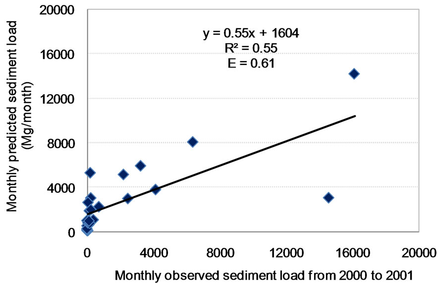
Figure 4. Model responses to monthly observed sediment load at Edinburgh (USGS 02482000) from January 2000 to December, 2001.
watershed (39.5 ha), which is a tributary of the Susquehanna River a part of the Chesapeake Bay in south central Pennsylvania [41]. The SWAT model predicted results were compared with monthly measured sediment concentration values from 1997 to 2004 with high resolution (field-specific management, row crop field); and low resolution (generic row crop field) scenarios. The model efficiency for the monthly sediment concentration prediction were reported varied (R2 values from 0 to 0.15; E values from –1.14 to –0.02) depending on the fields. The hydrologic impact due to longterm climate change (e.g. stream flow) was assessed from the UPRW using the SWAT model [21]. The model simulated results in the study indicated good model agreement (1981-2008) for mean monthly streamflow simulation (R2 from 0.69 to 0.79 and E from 0.68 to 0.79). The SWAT model peak flow results in his study demonstrated very close to ±10% range of the measured peak flow for the 42 peak flow events in the watershed. The results of the hydrologic simulations of this study agreed with the top 35% articles previously reviewed [17], which utilized the SWAT hydrologic model calibration and validation.
3.2. Bio-Energy Feedstock Yields
This study applied calibrated and validated SWAT model for the long-term (1998-2010) monthly stream flow. The model was further verified for the monthly sediment loads; and corn and soybean yields results within the watershed. Model simulations assessed feedstock and sediment yields responses of six bio-energy crops. Model simulated results of the six bio-energy crops were assessed from the selected pastureland and croplands (1669 km2) of the UPRW. The model simulated feedstock yields were compared for the two dominant Mississippi soils (MS048, and MS089) in the watershed. The MS048 and MS089 soils covered about 22.1% of the pastureland and cropland area in the watershed. The soil characteristics of MS048 soil include: fine sandy loam; distributed in the higher slope areas (8% - 12%); well drained soil with percentage fraction of clay 8.5%, silt 26.89%, and sand 64.61%; erodibility factor of 0.28; bulk density of 1.45 g/cm3. Similarly, the soil characteristics of MS089 soil include: silt loam; distributed in lower slope areas (0% - 8%); somewhat poorly drained soil with percentage fraction of clay 22.5%, silt 52.72%, and sand 24.78%; erodibility factor of 0.32; bulk density of 1.39 g/cm3.
There is no specific long-term continuous feedstock yield data available for the Miscanthus, Switchgrass, Johnsongrass, Alfalfa, Corn, and Soybean in the UPRW. However, Rankin County’s corn and soybean yield data was available for the period of 1998 to 2010 [42] except in 2002 and 2008 for soybean and 2008 and 2010 for corn to compare with the model simulated feedstock yields results. The crop yields data for the year 2002, 2008, and 2010 were utilized from the Madison County, a neighboring County within the watershed. The SWAT model simulated average annual corn and soybean yields from the selected land use and soil groups (369 km2) were compared with the twelve years (1997-2008) of Rankin County’s observed National Agriculture Statistics Service (NASS) annual average corn and soybean yields data.
The SWAT model reasonably predicted annual average corn yield (6.1 Mg/ha) when compared with the NASS county level observed annual average corn yield (6.8 Mg/ha) data (Figure 5(a)). Model predicted corn yield showed good correlation (R2 = 0.54) with the observed county level corn yield data. The SWAT model results determined that model under-predicted annual average corn yield by only 10%. Similarly, model predicted reasonable annual average soybean yield (2.4 Mg/ha) when compared with the NASS county level annual average soybean yield (2.2 Mg/ha) data (Figure 5(b)). Model predicted corn yield showed good correlation (R2 = 0.51) with the observed county level corn yield data. The SWAT model predicted results showed that model over-predicted annual average soybean yield by only 9%. The SWAT model predicted corn yield showed better correlation with observed data than soybean yield in this study as determined by R2 values (0.54 vs. 0.51) and regression slopes (0.62 vs. 0.33). The corn and soybean yields results of this study were found comparable with previous study using the SWAT model in the Lower Mississippi River Basin [25].
No compensation was given to corn and soybean or any other crops as this study was trying to assess relative feedstock yield potential and water quality benefits of the six bio-energy crops in the watershed using an equally treated management scenarios. Model uncertainty may exist due to localized crop management factors, errors associated with digital model input, observed crop yield,
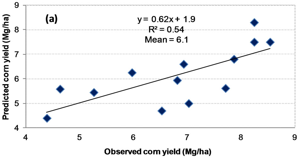
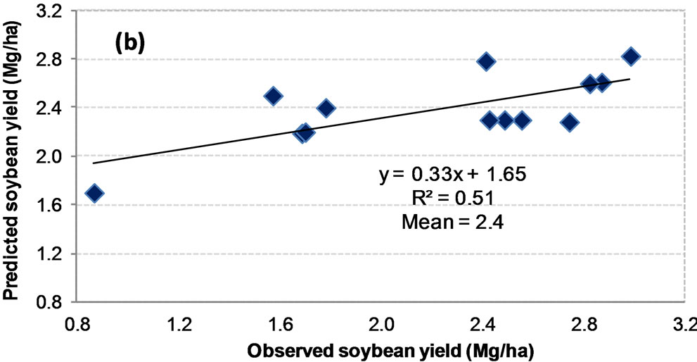
Figure 5. County level observed and model predicted (a) corn yield (Mg/ha) and (b) soybean yield (Mg/ha) from 1998 to 2010.
and spatial scale for the crop yield prediction. The SWAT model results are more likely affected by climate variability factors. Overall, the crop yield simulation results were found satisfactory considering the relative crop yield prediction for the comparison of six bio-energy feedstock yields and their water quality impacts in this study. In average feedstock yield from the MS048 soils had 1% greater than from the MS089 soils. When analyzing 13 years of annual average watershed feedstock yield results, Miscanthus grass determined the greatest feedstock yield from both MS048 and MS089 soils followed by Switchgrass, Johnsongrass, Alfalfa, Corn, and Soybean. Based on the model simulated feedstock yield results from two different soils (Table 2), it was estimated that the pastureland and cropland of the UPRW (369 km2) can produce 21.9 Mg/ha of average feedstock annually if Miscanthus grass is grown (Table 2). Similarly Switchgrass, Johnsongrass, Alfalfa, Corn, and Soybean can produce annual average feedstock yield of 15.2 Mg/ha; 12.1 Mg/ha; 7 Mg/ha; 5.9 Mg/ha; and 2.35 Mg/ha respectively (Table 2) from the UPRW.
Previous study applied SWAT model to assess the sustainability of producing Switchgrass as a bio-energy crop in a regional scale [23]. The Switchgrass yields predicted by the SWAT model varied from 0 Mg/ha in the northern US to over 16 Mg·ha–1 in southern Illinois, Arkansas, western Kentucky, and Tennessee in their study. Yields predicted across the southern extremes of the eastern US were reported typically between 6 and 12 Mg·ha–1. An empirical modeling tool was presented to simulate Switchgrass yields for the conterminous United States, which utilized geographically distributed field measured data [24]. Modeling tool over-predicted Switchgrass yields from the lowland agriculture when compared with the SWAT model predicted results. They have reported variations in the Switchgrass yields in the southwestern and northern margins as predicted by their empirical modeling tool. This study evaluated the UPRW conditions (soils: MS048 and MS089), which predicted long-term annual average Switchgrass yields of 15.2 Mg/ha.
Based on the SWAT model results, temporal distribution (1998-2010) of the feedstock yields followed the

Table 2. Model predicted average annual sediment and feedstock yields.
similar trends as long-term annual average watershed feedstock yield except for few years (Figure 6). The temporal affects on feedstock yields specially Miscanthus and Switchgrass could have been resulted due to the variation of climate change parameters, which impact on water stresses for each crop during model simulation period (1998-2010).
3.3. Water Quality and Evapo-Transpiration
Model simulated results determined that the corn crop scenario in the watershed had the greatest annual average sediment yield (12 Mg/ha) and the Miscanthus grass scenario had the least (1.1 Mg/ha) sediment yield. Annual average sediment yields from the MS048 soils were predicted greater than from the MS089 soils in the watershed as MS048 soil HRUs were spatially distributed in the higher slope range of the UPRW. The SWAT model simulation determined that annual average water yield difference of up to 7% from Miscanthus and soybean bio-energy crops scenarios in the watershed (Table 3). The model estimated results showed that Miscanthus crop had the greatest (532 mm) evapotranspiration (ET) demand and the soybean had the least (485 mm; Table 3). The SWAT model calculates actual ET, once total PET (1550 mm; Table 3) is determined and it evaporates any rainfall intercepted by the plant canopy.
The ET includes all the processes by which water from


Figure 6. Model simulated long-term (28 years) average annual feedstock yield (Mg/ha) of the six bio-energy crops from the two Mississippi soils (a) 048 and (b) 089 during the study period in the watershed.
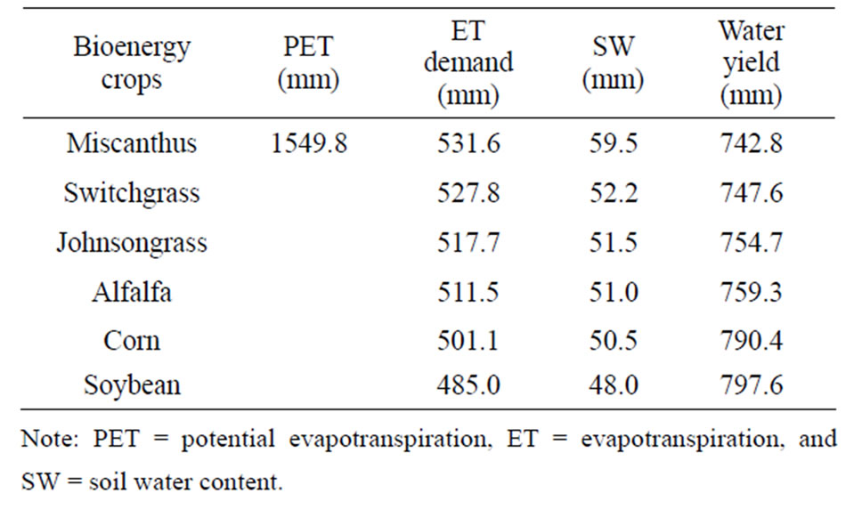
Table 3. Estimated annual average PET, ET, and water yield for bio-energy crops.
the surface of the ground is changed to water-vapor (e.g. from soil and plant-canopy, transpiration). This study selected the Penman-Monteith method in the model to estimate PET from the watershed. The Penman-Monteith method in the SWAT model considers evaporation, water vaporization mechanisms, aerodynamic and surface resistance terms [28]. In the SWAT model crop-yield is determined based on the amount of dry-biomass above the ground and harvest index, which is calculated daily during the plant growing season [28]. The duration of the crop period of each bio-energy crops are varied. In this study, Miscanthus had 47 mm greater ET demand than that of soybean. In addition, Miscanthus holds annual average of about 12 mm greater soil water (SW) than soybean (59.5 mm vs. 48 mm in Table 3), which means about 11% less annual surface water flow from the watershed could be anticipated when converting land area from soybean to Miscanthus. The SWAT model results determined that annual average SW holding from Miscanthus greater than Switchgrass and Corn crops. The SWAT model predicted annual average ET from the Switchgrass crop greater than the corn and soybean crops (Table 3), which was anticipated based on the crop parameters used in the Table 1; and SWAT model database [28]. The results of this study showed consistency with previous literatures [43]. Modeling results of this study suggested that the more corn and soybean production in the watershed will reduce annual ET resulting in the greater amount of water and sediment yields. In contrast, more pasturelands in the watershed will increase ET resulting in the less amounts of water and sediment yields from the watershed. The relative model simulated results presented in this study are good for making comparisons and water management evaluations.
4. Conclusions
The main objective of this study was to compare potential bio-energy crops production and their impact on water quality within the UPRW. Individual feedstock yields from two soil groups investigated in this study (MS048 and MS089) were found slightly different (MS048 higher) as determined by the SWAT model. Miscanthus grass predicted consistently higher feedstock yield than other bio-energy crops from both soils compared in this study. Annual average sediment yield from the MS048 soils predicted 145% greater than from the MS089 soils in the watershed as MS048 soils were distributed in the higher slope range of the HRUs in the watershed.
Overall, model simulated long-term annual average feedstock yield results from the UPRW determined the greatest when growing Miscanthus grass followed by Switchgrass, Johnsongrass, Alfalfa, Corn, and Soybean. Miscanthus grass simulated in this study can produce about 63% greater feedstock quantity than Switchgrass and 79% feedstock quantity than Johnsongrass. Feedstock yields of the bio-energy crops investigated in this study could vary depending up on application of fertilizer rates and soil water moisture conditions. The bio-energy crops Alfalfa, Corn, and Soybean determined the least three crops producing feedstock. Model simulated results determined that the corn crop scenario in the watershed had the greatest annual average sediment yield (12 Mg/ha) and the Miscanthus grass scenario had the least (1.1 Mg/ha) sediment yield. Modeling results also suggested that increased corn and soybean crop cultivation in the watershed will reduce annual average ET, which increases water and sediment yields from the watershed. In contrast, increase in the grasslands acreage in the watershed will increase annual average ET and reduce water and sediment yields from the watershed. About 11% less annual average surface water flow from the watershed could be anticipated when converting land areas from soybean to Miscanthus grass. The SWAT model simulated results suggested that growing Miscanthus grass in the UPRW would have the greatest feedstock source for bio-energy and water quality benefits. Results of this study are relevant to the active management of water in agriculture in view of growing land use change for bioenergy needs.
5. Acknowledgements
This material is based upon work performed through the Sustainable Energy Research Center at Mississippi State University and is supported by the Department of Energy under Award Number DE-FG3606GO86025; Micro CHP and Bio-fuel Center; and Special Research Initiatives (SRI) and the Mississippi Agricultural and Forestry Experiment Station (MAFES). We acknowledge the contributions of Mr. Kurt Readus, area conservationist, NRCS/MS.
REFERENCES
- US Energy Information Administration (EIA), “World Energy Consumption and Carbon Dioxide Emissions, 1990-2025,” 2004-2005. http://www.infoplease.com/ipa/A0776146.html
- US Energy Information Administration (EIA), “U.S. Carbon Dioxide Emissions in 2009: A Retrospective Review,” 2009. http://www.eia.gov/oiaf/environment/emissions/carbon/pdf/2009_co2_analysis.pdf
- US Department of Energy (US/DOE), “Energy Information Administration Annual Energy Outlook,” Report No. DOE/EIA-0383, National Energy Information Center, Washington DC, 2004, pp. 1-221.
- US Census Bureau (USCB), “International Database,” 2011. http://www.census.gov/ipc/www/popclockworld.html
- J. Hill, E. Nelson, D. Tilman, S. Polasky and D. Tiffany, “Environmental, Economic, and Energetic Costs and Benefits of Biodiesel and Biofuels,” Proceedings of the National Academy of Sciences, Vol. 103, No. 30, 2006, pp. 11206-11210. doi:10.1073/pnas.0604600103
- J. Milliken, F. Joseck, M. Wang and E. Yuzugullu, “The Advanced Energy Initiative,” Journal of Power Sources, Vol. 172, No. 1, 2007, pp. 121-131. doi:10.1016/j.jpowsour.2007.05.030
- D. Pimentel, and T. W. Patzek, “Ethanol Production Using Corn, Switchgrass and Wood; Biodiesel Production Using Soybean and Sunflower,” Natural Resources Research, Vol. 14, No. 1, 2005, pp. 65-76. doi:10.1007/s11053-005-4679-8
- S. C. Davis and S. W. Diegel, ”Transportation Energy Data Book,” ORNL-6973, Edition 24, Oak Ridge National Laboratory, Oak Ridge, 2004, pp. 1-348.
- W. T. W. Woodward, “The Potential for Alfalfa, Switchgrass and Miscanthus as Biofuel Crops in Washington,” Proceedings of the Washington State Hay Growers Association Annual Conference and Trade Show, Three Rivers Convention Center, Kennewick, 16-17 January 2008, pp. 1-7.
- B. Baldwin, “Biomass Energy Crops for the Southeast,” Biofuels Conference, Mississippi State University, Jackson, 12-13 August 2010.
- L. Wright, “Historical Perspective on How and Why Switchgrass Was Selected as a Model High-Potential Energy Crop,” Consultancy Work to Bioenergy Resources and Engineering Systems, ORNL/TM-2007/109, Oak Ridge National Laboratory, 2007, pp. 1-59.
- S. B. McLaughlin and L. A. Kaszos, “Development of Switchgrass as a Bioenergy Feedstock in the United States,” Biomass Bioenergy, Vol. 28, 2005, pp. 515-535. doi:10.1016/j.biombioe.2004.05.006
- J. E. King, J. M. Hannifan and R. G. Nelson, “An Assessment of the Feasibility of Electric Power Derived from Biomass and Waste Feedstocks,” Report No. KRD- 9513, Kansas Electric Utilities Research Program and Kansas Corporation Commission, Topeka, 1998, pp. 1- 266.
- US Environmental Protection Agency (EPA), “National Summary of Impaired Waters and TMDL Information,” US Environmental Protection Agency, Washington DC, 2010. http://iaspub.epa.gov/waters10/attains_nation_cy.control?p_report_type=T
- J. R. Williams, “The EPIC Model in Computer Models of Watershed Hydrology, Chapter 25,” Water Resources Publications, Highlands Ranch, 1995, pp. 909-1000.
- J. G. Arnold, R. Srinivasan, R. S. Muttiah and J. R. Williams, “Large Area Hydrologic Modeling and Assessment Part I: Model Development,” Journal of American Water Resource Association, Vol. 34, No. 1, 1998, pp. 73-89. doi:10.1111/j.1752-1688.1998.tb05961.x
- P. W. Gassman, M. R. Reyes, C. H. Green and J. G. Arnold, “The Soil and Water Assessment Tool: Historical Development, Applications, and Future Research Directions,” Transactions of the ASABE, Vol. 50, No. 4, 2007, pp. 1211-1250.
- P. B. Parajuli, K. R. Mankin and P. L. Barnes, “Applicability of Targeting Vegetative Filter Strips to Abate Fecal Bacteria and Sediment Yield Using SWAT,” Agricultural Water Management, Vol. 95, No. 10, 2008, pp. 1189- 1200. doi:10.1016/j.agwat.2008.05.006
- P. B. Parajuli, K. R. Mankin and P. L. Barnes, “Source Specific Fecal Bacteria Modeling Using Soil and Water Assessment Tool Model,” Bioresource Technology, Vol. 100, No. 2, 2009, pp. 953-963. doi:10.1016/j.biortech.2008.06.045
- M. S. Kang, S. W. Park, J. J. Lee and K. H. Yoo, “Applying SWAT for TMDL Programs to a Small Watershed Containing Rice Paddy Fields,” Agricultural Water Management, Vol. 79, No. 1, 2006, pp. 72-92. doi:10.1016/j.agwat.2005.02.015
- P. B. Parajuli, “Assessing Sensitivity of Hydrologic Responses to Climate Change from Forested Watershed in Mississippi,” Hydrological Processes, Vol. 24, No. 26, 2010, pp. 3785-3797. doi:10.1002/hyp.7793
- R. G. Nelson, J. C. Ascough II and M. R. Langemeier, “Environmental and Economic Analysis of Switchgrass Production for Water Quality Improvement in Northeast Kansas,” Journal of Environmental Management, Vol. 79, No. 4, 2006, pp. 336-347. doi:10.1016/j.jenvman.2005.07.013
- L. Baskaran, H. I. Jager, P. E. Schweizer and R. Srinivasan, “Progress toward Evaluating the Sustainability of Switchgrass as a Bioenergy Crop Using the SWAT Model,” Transactions of the ASABE, Vol. 53, No. 5, 2010, pp. 1547-1556.
- H. I. Jager, L. Baskaran, C. C. Brandt, E. Davis, C. A. Gunderson and S. Wullschleger, ”Empirical Geographic Modeling of Switchgrass Yields in the United States,” GCB Bioenergy, Vol. 2, 2010, pp. 248-257. doi:10.1111/j.1757-1707.2010.01059.x
- R. Srinivasan, X. Zhang and J. Arnold, “SWAT Ungaged: Hydrological Budget and Crop Yield Predictions in the Upper Mississippi River Basin,” Transactions of the ASABE, Vol. 53, No. 5, 2010, pp. 1533-1546.
- R. L. Huhnke, J. F. Stritzke and J. B. Solie, “Primary Tillage Effects on Alfalfa Establishment and Yield,” Transactions of the ASAE, Vol. 9, No. 6, 1993, pp. 495- 499.
- S. L. Dillard, “Productivity and Nutritive Quality of Johnsongrass as Influenced by Interseeded Ladino Cover and Fertilization with Commercial Fertilizer or Broiler Litter,” MS Thesis, Auburn University, Auburn, 2009.
- S. L. Neitsch, J. G. Arnold, J. R. Kiniry and J. R. Williams, “Soil and Water Assessment Tool (SWAT), Theoretical Documentation,” Blackland Research Center, Grassland, Soil and Water Research Laboratory, Agricultural Research Service, Temple, 2005.
- US Geological Society (USGS), “National Elevation Dataset,” 1999. http://seamless.usgs.gov/website/seamless/viewer.htm
- US Department of Agriculture (USDA), “Soil Data Mart,” Natural Resources Conservation Service, 2005. http://soildatamart.nrcs.usda.gov/Default.aspx
- US Department of Agriculture, National Agricultural Statistics Service (USDA/NASS), “The Cropland Data Layer,” 2009. http://www.nass.usda.gov/research/Cropland/SARS1a.htm
- National Climatic Data Center (NCDC), “Locate Weather Observation Station Record,” 2012. http://www.ncdc.noaa.gov/oa/climate/stationlocator.html
- J. M. O. Scurlock, “Miscanthus: A Review of European Experience with a Novel Energy Crop,” Environmental Sciences Division, Publication No. 4845, Oak Ridge National Laboratory Oak Ridge, 2009.
- T. L. Ng, J. W. Eheart, X. Cai and F. Miguez, “Modeling Miscanthus in the Soil and Water Assessment Tool (SWAT) to Simulate Its Water Quality Effects as a Bioenergy Crop,” Environmental Science and Technology, Vol. 44, No. 18, 2010, pp. 7138-7144. doi:10.1021/es9039677
- E. A. Heaton, F. G. Dohleman and S. P. Long, “Meeting U.S. Biofuel Goals with Less Land: The Potential of Miscanthus,” Global Change Biology, Vol. 14, 2008, pp. 2000-2014. doi:10.1111/j.1365-2486.2008.01662.x
- R. L. Hall, “Grasses for Energy Production Hydrological Guidelines,” B/CR/00783/Guidelines/Grasses.URN 03/ 882, Centre for Ecology and Hydrology, 2003.
- D. N. Moriasi, J. G. Arnold, M. W. Van Liew, R. L. Bingner, R. D. Harmel and T. L. Veith, “Model Evaluation Guidelines for Systematic Quantification of Accuracy in Watershed Simulations,” Transactions of the ASABE, Vol. 50, No. 3, 2007, pp. 885-900.
- A. Y. Sheshukov, C. B. Siebenmorgen and K. R. Douglas-Mankin, “Seasonal and Annual Impacts of Climate Change on Watershed Response Using an Ensemble of Global Climate Models,” Transactions of the ASABE, Vol. 54, No. 6, 2011, pp. 2209-2218.
- A. P. Nejadhashemi, S. A. Woznicki and K. R. DouglasMankin, “Comparison of Four Models (STEPL, PLOAD, L-THIA, AND SWAT) in Simulating Sediment, Nitrogen, and Phosphorus Loads and Pollutant Source Areas,” Transactions of the ASABE, Vol. 54, No. 3, 2011, pp. 875-890.
- P. B. Parajuli, N. O. Nelson, D. F. Lyle and K. R. Mankin, “Comparison of AnnAGNPS and SWAT Model Simulation Results in USDA-CEAP Agricultural Watersheds in South-Central Kansas,” Hydrological Processes, Vol. 23, No. 5, 2009, pp. 748-763. doi:10.1002/hyp.7174
- T. L. Veith, A. N. Sharpley and J. G. Arnold, “Modeling a Small Northeastern Watershed with Detailed, FieldLevel Data,” Transactions of the ASABE, Vol. 51, No. 2, 2008, pp. 471-483.
- US Department of Agriculture, National Agricultural Statistics Service (USDA/NASS), “County Estimates,” 2011. http://www.nass.usda.gov/Statistics_by_State/Mississippi/Publications/County_Estimates/index.asp
- K. E. Schilling, M. K. Jha, Y. K. Zhang, P. W. Gassman and C. F. Wolter, “Impact of Land Use and Land Cover Change on the Water Balance of a Large Agricultural Watershed: Historical Effects and Future Directions,” Water Resources Research, Vol. 44, No. 7, 2008, pp. 1- 12.