Journal of Water Resource and Protection
Vol.3 No.10(2011), Article ID:8137,13 pages DOI:10.4236/jwarp.2011.310087
Inexpensive Geophysical Instruments Supporting Groundwater Exploration in Developing Nations
1Department of Geology and Environmental Science, Wheaton College, Wheaton, Illinois, USA
2Design Engineer, Wheaton, Illinois, USA
E-mail: james.clark@wheaton.edu
Received June 16, 2011; revised August 7, 2011; accepted September 12, 2011
Keywords: Groundwater Geophysics, Inexpensive, Developing World, Resistivity, Seismic Refraction, Groundwater Exploration
ABSTRACT
Geophysical methods are often used to aid in exploration for safe and abundant groundwater. In particular resistivity and seismic refraction methods are helpful in determining depth to bedrock and zones of saturation in the subsurface. However the expense of these instruments ($5000 to $20,000) has resulted in their limited use in developing countries. This paper describes how to construct these devices for less than $250 each. The instruments are small, light and robust and are as useful for groundwater exploration as the commercial models for shallow aquifers (less than 35 m deep) where wells can be hand dug, augured or drilled with small portable drill rigs. Data interpretation can be accomplished quickly in the field with free software implemented on a laptop computer. A suite of geophysical instruments and software can therefore be assembled for less than $850. This paper gives the design for these instruments and essential information needed to use them. It is hoped that these inexpensive geophysical instruments can be widely distributed among drillers and aid workers in developing countries, improving the success rate of water wells.
1. Introduction
Because the need for safe water in much of Africa and many developing nations is so great and sustainable water production is desired, training of a host of indigenous workers with skills to drill, develop, complete and maintain good wells is essential. To this end a team from LifeWater International trained an effective team of Tanzanians to drill and complete shallow wells (<35 m deep) with a small portable drill rig (LS-100). This mud rotary rig can drill quickly through soft and unconsolidated sediments, but cannot penetrate the hard crystalline bedrock common in East Africa. During the following year the highly productive indigenous team drilled 50 boreholes but, because there was little geological rationale for siting each well other than avoiding proximity to sources of contamination, 15 of those wells were dry. The aquifer in the southern highlands of Tanzania is slightly weathered granite or gneiss found immediately above unweathered bedrock, but below 5 to 40 m of clay. Dry boreholes typically occurred where bedrock was close to the surface (<10 m) so that the water table was below the permeable weathered zone, or where bedrock was so deep (>35 m) that the aquifer was beyond the depth limit of the small drill rig. Similar depth limits constrain hand auger drilling methods and hand-dug wells. Prior knowledge of the approximate depth to bedrock would be extremely valuable information aiding the selection of drilling sites in this region.
In a different geological regime villagers in eastern Chad hand-dig shallow wells, 1.5 to 3 meters deep, in the sands of wadis to provide their families with water for 6 months of the year. During the dry season the water table drops below the bottom of the wells and the women must travel several kilometers to obtain water from large dry sandy river beds. Hard crystalline bedrock limits the depth of the wells, but its surface is highly irregular so that overlying sand thicknesses differ dramatically over short distances. Knowledge of the approximate depth to bedrock would enable wells to be dug in thick sand sequences which remain saturated throughout much of the year.
In each of these cases the striking contrast in physical properties between the overlying unconsolidated material, clay or sand, and the hard bedrock makes geophysical methods particularly attractive as a means of detecting depth to bedrock. In particular, the well known electrical resistivity and seismic refraction techniques are very well suited to determination of depth to bedrock under these geological situations [1]. In the resistivity method a slowly alternating electrical current flows through the ground, such that, through analogy to Ohm’s law (resistance = voltage/current), measurement of voltage and current at the ground surface gives an estimate of the electrical resistance in the subsurface. Because the electrical resistance is related to lithology and saturation, the subsurface geological conditions can be estimated. In the seismic refraction method sound waves produced by an explosion or sudden shock at the surface travel through the subsurface. Shock waves travel much faster in bedrock than in unconsolidated material and, in analogy to Snell’s law of optics, eventually refract back towards the surface. Accurate measurement of initial arrival times of these refracted waves allow inference of depth to bedrock layers.
These techniques using commercially available instruments have been shown to be very helpful in finding water in Africa. In one study of 370 wells drilled in Zimbabwe the use of resistivity surveys improved the success rate for wells from 50% to 85 % [2]. Kirsch [3] provides an overview of geophysical methods in support of groundwater exploration, and in that volume Rabbel [4] considers seismic and resistivity methods as second only to drilling for usefulness in determining the subsurface structure. His paper also explains that both methods should be used for maximum information because they complement each other.
This paper will add little to the immense literature about the theory, use, and interpretation of resistivity and seismic refraction methods developed over the past 70 years in support of oil exploration and, more recently, groundwater exploration [3,5]. The objective is to demonstrate that instruments costing tens of thousands of dollars if purchased commercially can be constructed for less than $250. Such inexpensive tools could be disseminated widely among drillers who could use them to determine depth to bedrock, and therefore increase the chance of completing successful water wells. Thus the instruments would be operated not by highly-paid consultants or a few geologists employed by governments but by those who are actually drilling wells. Although these instruments are much less elaborate than the commercial models, they are capable of similar accuracies where prospecting targets are shallow. They are much less cumbersome to transport and easier to repair under field conditions than commercial units. Furthermore, if an inexpensive laptop computer is available, free software can be used to interpret the geophysical data while in the field. However, commercial models typically allow more efficient data collection and commercial software provides more refined data interpretation.
Others have reported developing inexpensive resistivity [6] and seismic instruments [7] for educational purposes, but the use of similar instruments for water prospecting in developing countries has not been addressed. Olowofela et al. [8] working in Nigeria have recently outlined the plans for a resistivity meter in the context of physics research, but their plans are more elaborate than those proposed by us and have not been applied specifically to water prospecting.
The following sections briefly describe the theory of each technique in turn and then outline construction and interpretation procedures. Each section concludes with an application of the technique to the geological situations outlined above for Tanzania and Chad.
2. Resistivity Method
It is not necessary to review in detail the theoretical basis for “vertical electrical sounding (VES)” because, for all but the simplest homogeneous earth model, the theory is difficult and adds little to meeting the objectives of this paper. A brief discussion of the theory and field methods, however, is important to understand the rationale for features included in the instrument and data interpretation method.
2.1. Theory
A DC voltage across two current electrodes (A, B) inserted into soil causes an electrical current to flow through the ground (Figure 1). Potential electrodes (M, N) are inserted between and in line with the current electrodes. Measurements of the electrode spacing, the current (I) and the voltage drop between the potential electrodes (Vm) are made and then the electrode spacing is increased and the measurement repeated. As the electrode spread increases, the depth of penetration of the current increases so the surface readings become more affected by electrical properties at depth. The electrical property of interest is ground resistivity with units given in ohm-meters.
Two electrode configurations are common (Figure 2). In the Wenner arrangement the spacing between each electrode, “a”, is constant. When the current electrodes are moved farther apart to induce a deeper current, the inner potential electrodes must also be moved. With the Schlumberger method the potential electrodes remain fixed and only the outer current electrode spread increases.
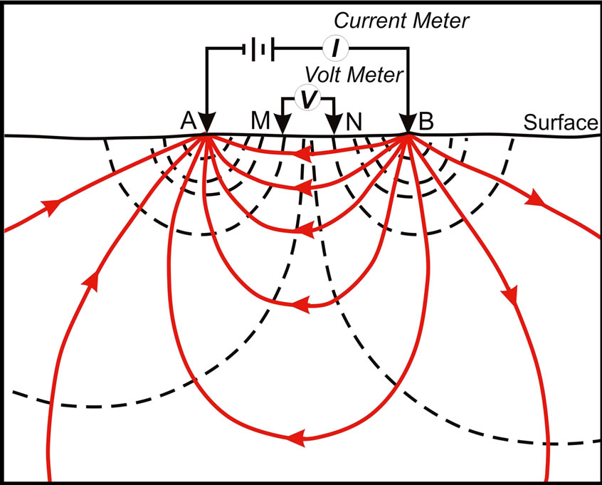
Figure 1. Schematic illustration of the resistivity method. Solid red lines represent current flow. Dashed black lines contour electrical potential (voltage).
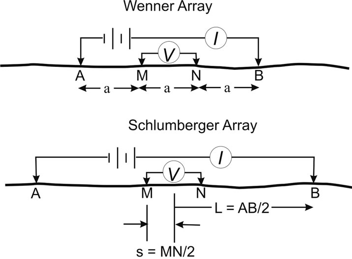
Figure 2. The two most common electrode configurations.
The measurements of I and Vm are used to calculate the “apparent resistivity,” which is the resistivity for the equivalent homogeneous earth that produces the same I and Vm. For the Wenner electrode configuration the apparent resistivity is
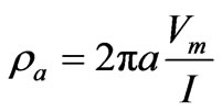 . (1)
. (1)
For the Schlumberger arrangement the relationship is
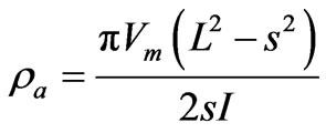 (2)
(2)
with the L and s distances defined in Figure 2. For a homogeneous earth structure, as the current electrodes are spread farther apart the apparent resistivity will not change. If the actual earth resistivity decreases with depth, as often occurs in Tanzania, the calculated apparent resistivity will decrease as the electrode spread increases. This occurs because at large spread a greater proportion of current is flowing in the lower resistivity region at depth, and that is reflected in the measured current and voltage at the surface. It is this relationship, coupled with theory of current flow in layered materials, that allows inference of resistivity properties at depth.
Two problems can arise in that 1) the earth may have a natural voltage or “self potential” that is unrelated to earth resistivity at depth, and 2) the DC current source itself can gradually induce an electrical potential around the electrodes from polarization. Both the self potential and the induced polarization effects can be minimized by periodically reversing the current at a rate of about 1 Hertz. A slowly alternating current reduces polarization because a charge concentration cannot accumulate. If VSP is the natural ambient earth self-potential, assumed to be constant, and Vp is the voltage induced by the current electrodes, then the measured voltage, Vm, across the potential electrodes is
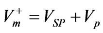 . (3)
. (3)
If the current is reversed only the Vp voltage is affected by the sign change so that the reading is then
 . (4)
. (4)
The difference in the pair of readings gives 2Vp and half this difference is then the desired Vp. In the field it is convenient to use reversing switches for both the current and the potential reading. If both are switched simultaneously, the measured voltage values only need to be added rather than subtracted, and the average of the measurements is then Vp. At the African sites described above the average of four values of voltage and current is adequate and reproducible. More readings can be averaged, but there must be an even number of measurements to ensure that the VSP term is eliminated.
2.2. Construction
Commercial resistivity devices are excellent, and they now contain microprocessors that control current reversal and averaging procedures and even calculate apparent resistivity for each standard electrode configuration. They are also expensive ($5000 to $10,000) and repair is costly and time-consuming. The design goal was to build a resistivity device for less than $250 because then it could remain with the LS-100 drill rig for national drill team use. Further requirements were simplicity, so that repair in the field is possible, and robustness so that repair would not be needed even under harsh African conditions. Furthermore, because of airline transport issues, it had to be light, compact, and with no large batteries, which are now prohibited on many flights. Because of ready availability in almost any country, a 12-volt car battery was used as the power source. A small commercially available 400 watt inverter that produces an AC “modified” sine wave from a 12 volt DC source was used to increase the voltage to the required value of several hundred volts. A full-wave bridge rectifier in parallel with a 1 μF capacitor converts the AC voltage to a high steady DC voltage. The inverter used in Tanzania had a 120 volt AC output producing a DC voltage output from the resistivity device under no load of 170 volts. A high voltage across the current electrodes is desired because the maximum spread, and hence the depth of current penetration in the ground, is limited by the voltage magnitude across the current electrodes. In Tanzania resistivities at depths exceeding 35 m were barely detected. An even higher DC voltage is needed for the Schlumberger electrode array because the potential electrodes are not widely spaced and so have a lower voltage drop across them than the equivalent Wenner array. An identical device built upon return from Tanzania uses a commercial inverter that produces 240 volts AC, resulting in a DC no-load voltage of 330 volts. An added benefit of the inverter is that it can provide power in the field for a laptop computer, useful in data interpretation.
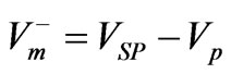
The electrical schematic (Figure 3) includes two reversing switches (DPDT)—one for the ammeter and one for the voltmeter. To measure the current and voltage two small inexpensive digital multimeters worked well. For U.S. applications filtering AC noise is important, but in Tanzania that problem did not exist as no electricity was close to the drill sites. The isolation from electrical noise in developing countries is a great advantage. The four electrodes were 10-inch lag screws, and were attached with large alligator clips to stranded single conductor 14-gauge house wire which was cheaper than the lighter 18 gauge wire used in commercial devices. Two 152 m (500 feet) spools of house wire will allow a maximum current electrode spread with the Wenner array of 228 m (750 feet), and would be adequate for almost any survey. From each spool cut off 38 m (125 feet) for the
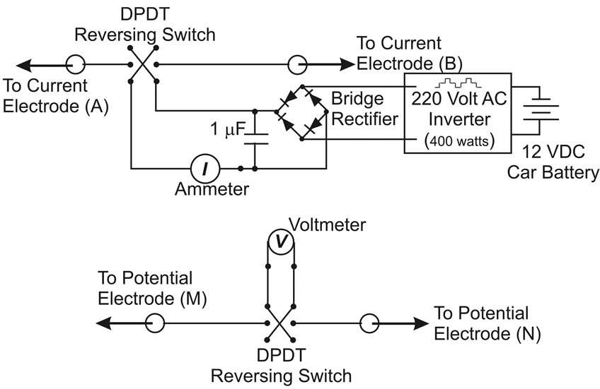
Figure 3. Electrical circuit used in the inexpensive resistivity device.
potential electrodes. Two tape measures, preferably more than 60 m long, to extend in both directions from the array center are the only additional equipment needed for a survey.
The total cost (Table 1) of $206 is well within the design budget. Most of the materials can be obtained from electronic supply and hardware stores. The 220 VAC inverter and the inexpensive multimeters were purchased from internet sources. Pictures of the unit and the field arrangement (Figures 4 (a), (b)) illustrate how small and simple it is. Tests of the device at Northern Illinois University confirmed that results were virtually identical to
 (a)
(a)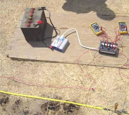 (b)
(b)
Figure 4. (a) Resistivity instrument exterior and (b) field setup at Mgongo, Tanzania.
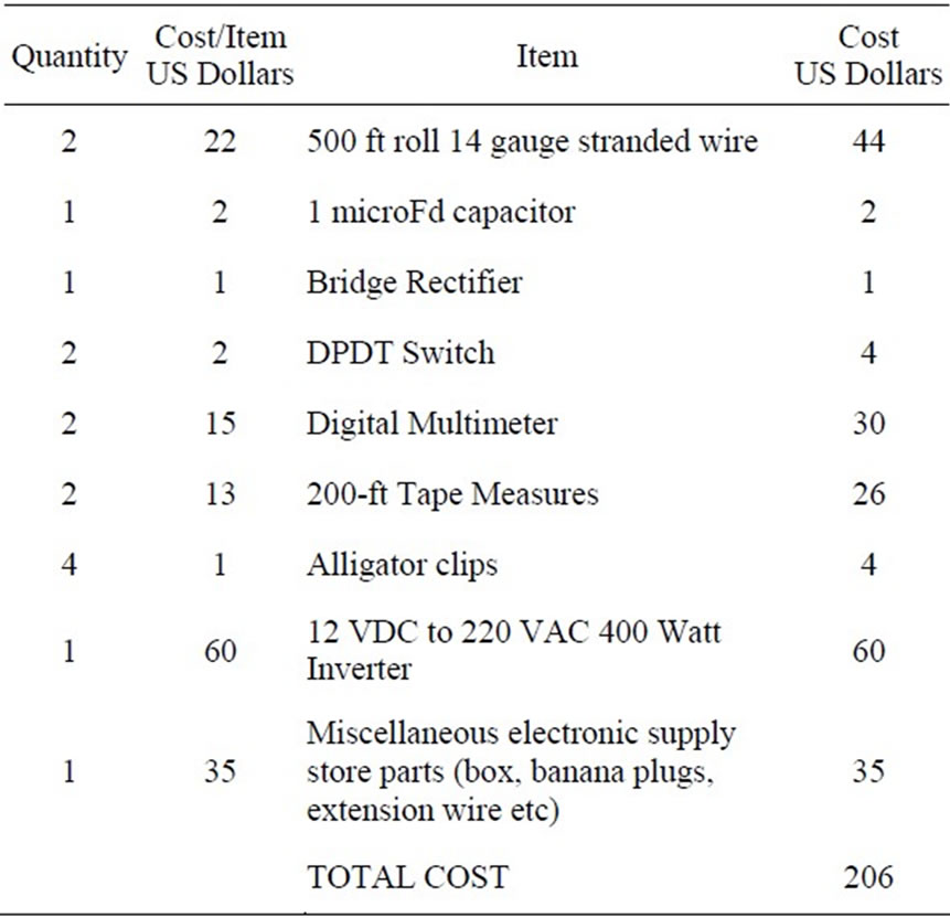
Table 1. Itemized list of resistivity device materials and cost.
those from a commercial $10,000 resistivity instrument (Sting R1), though the commercial instrument provided apparent resistivity values instantaneously whereas the values for ρa for our instrument had to be calculated from the current and voltage readings using Equation (1). A test in Nigeria with another Sting R1 resistivity instrument validated the accuracy of the inexpensive instrument (Figure 5).
2.3. Field Method
For efficient surveying at least 3 people are needed to operate the instrument and insert the electrodes, but conceivably only one operator is necessary. Once a site is selected the two tape measures are extended outward and the electrodes inserted symmetrically about the center. When the battery, inverter, and multimeters are connected to the resistivity device and the wires are attached to the electrodes, readings can commence. In the Tanzanian field area annual rainfall is 91 cm, but during 6 months of the year only 6 cm is typical and the soil is very dry. A serious error can occur if any electrode does not have a good electrical contact with the soil and so water was poured into a small shallow hole, made with a hammer, to saturate the ground near each electrode. The electrode was then pounded into the saturated ground. The reversing switches are thrown manually, and the ammeter and voltmeter readings taken after a brief delay to allow values to stabilize. The switches were thrown four times and an average calculated for voltage and current.
The Schlumberger configuration is much faster and easier to implement in the field, but when the current electrodes are very far apart (e.g. 100 m) the voltage Vm may be too small to detect reliably. In that case the potential electrodes must be spread farther apart without
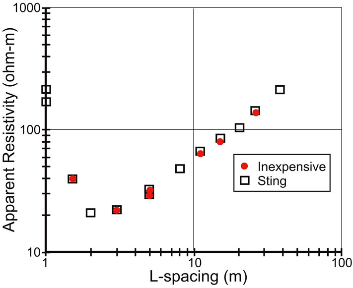
Figure 5. Apparent resistivity comparison between the commercial resistivity meter Sting R1 and the inexpensive resistivity instrument. Results are very similar.
moving the current electrodes and another reading taken. Normally some slight offset in ρa values occurs, and this requires adjustment during interpretation. It is best to keep the spacing of the current electrodes more than 5 times the potential electrode spacing. The Wenner array always has maximum potential electrode spacing, and therefore would be more appropriate where the depths investigated are near the limit of the instrument. It is helpful to have a tabulated chart of the location of the electrodes for different Wenner “a” spacing. This is not necessary for the Schlumberger spread. After each reading the spread is increased until the instrument readings exceed the accuracy of the multimeters. This typically occurred at a 90 m spread with the 120 volt AC inverter.
2.4. Data and Results
Using the inexpensive resistivity instrument and a Wenner electrode spacing geometry, the Tanzanian drill team collected data at three sites (Figure 6). Wells already existed at two of the sites and they planned to drill a borehole at the third (Mafinga). Data from all VES indicate that apparent resistivity decreases as the current penetrates deeper into the ground with increasing Wenner “a-spacing.” At an a-spacing that differs among all surveys, apparent resistivity starts to increase, suggesting that at depth there is a resistivity increase. It is clear that the a-spacing at the minimum apparent resistivity value is related to bedrock depth.
Computer software for resistivity interpretation is readily available commercially. These codes can be very elaborate and often include the possibility of predictions of both vertical and horizontal changes in resistivity. This software is expensive. If the goal is to find only vertical variation in resistivity and one is content to assume that the layer interface is horizontal (or at least dipping less than 15 degrees) then free software can be used. In Tanzania freeware provided by Dr. Philip Carpenter of Northern Illinois University was used. It followed the theory of Ghosh [9,10] and required the DOS operating system. The simplest resistivity model that fits the Tanzanian data has three layers and gives an acceptable estimate of the depth to bedrock. It is possible to estimate geological materials from resistivity values (Table 2), but the large range in the values makes such estimates approximate. In this region surface clay is dry to a depth of a few meters. Below that the clay is saturated and of very low resistivity, but its extremely low permeability precludes it as an aquifer. Below the clay is bedrock that is essentially an electrical insulator halfspace of several thousand ohm-m. The fit to the data at the Mafinga site (Figure 6) resulted in the interpretation that depth to bedrock is approximately 30 meters. The
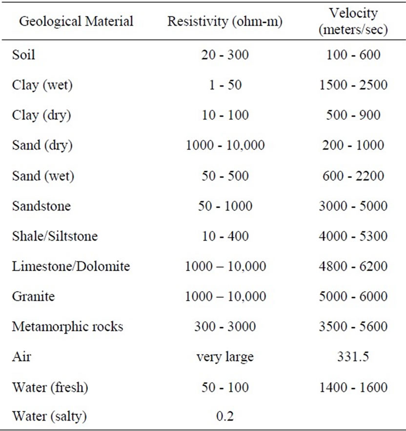
Table 2. Typical Geophysical Properties (from [7,13-15] and [1] pp. 452-456).
upper layer is 1.5 m thick with resistivity of 110 ohm-m, and overlies a 29 m layer with 6.5 ohm-m resistivity. The substrate halfspace is at least 2000 ohm-m, which is essentially a perfect insulator. The curves in Figure 7 represent models with these resistivities where only the thickness of the middle layer is changed. Where the geological materials are similar, the depth can be estimated by the a-spacing value at the minimum point of the curve. Comparison of predictions to the data clearly rules out depths to bedrock, and the overlying aquifer, less than 15 m, which would be too shallow and wells would likely dry up during part of the year. So the well was drilled and reached bedrock at 28 meters. Water from the aquifer of slightly weathered bedrock underlying the clay rose in the well to within 5 m of the surface, and a high yield well was completed.
2.5. Discussion
The Tanzanian drill team quickly learned how to perform the field operations, but navigating the DOS operating system was daunting. We subsequently developed user friendly software for the Windows operating system to calculate apparent resistivities. It also provides a Monte Carlo method to invert the observed apparent resistivities for the likely lithologic thicknesses. The Schlumberger geometry is more efficient in the field than the Wenner configuration, but a greater input voltage is needed to penetrate to the same depth because the potential electrodes are closer together, and so are sampling a smaller
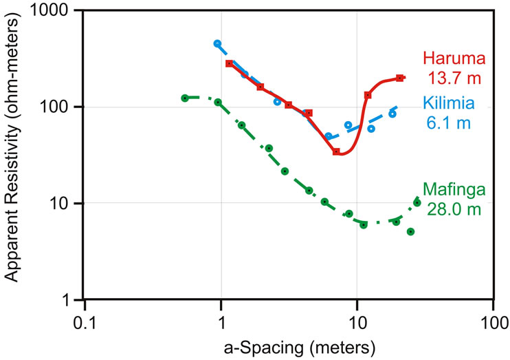
Figure 6. Resistivity data at three sites with known depth to bedrock given.
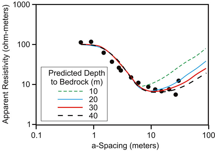
Figure 7. Mafinga resistivity data compared to predictions at differing predicted depths to bedrock. Depths of 20 to 30 m fit best. Actual bedrock was at 28 m depth.
range of voltage. Both a Schlumberger and a Wenner array were used at one locality (Mgongo), and the final interpretation from the two methods was similar.
Data collection typically took about two hours, but learning and training was occurring simultaneously. It is estimated that three trained workers can do a survey in about one hour, including the interpretation, if a laptop computer is available. This provides quick and useful screening to detect if basement rock is too close to the surface. Most of the field time was spent in measuring and moving the electrodes, so, relative to the Wenner approach used in the Tanzanian study, the Schlumberger method would halve the field time as only the two current electrodes are moved for each reading. For bedrock depths approaching 30 m the voltage source (120 VAC or 170 VDC) was near its limit. Use of the 220 VAC (400 watt) inverter would double the DC voltage output and make interpretations down to 35 m depth more reliable. A higher voltage is necessary for the Schlumberger approach because the closer spacing of the potential electrodes results in a smaller voltage drop. It would be easy and cheap (<$10) to add a small instrument amplifier chip (up to 50× voltage amplification) to allow more precise readings when the voltages are in the 5 to 10 millivolt range. It is not clear, however, whether noise in the environment and from the inverter would mask the signal.
The software allows rapid fitting of the resistivity model to the data, but, as with most geophysical techniques, the resulting resistivity model is not unique. Because of errors in the data and physical trade-offs (e.g. thicker layer but lower resistivity vs thinner layer but higher resistivity), it is possible to fit the data within its errors with different geologic models. With experience in a given geological regime an operator will likely be able to recognize and eliminate unlikely models.
If no computer is available it is still possible to interpret the data using the “Master Curve” method. This method was used in the 1960’s to interpret resistivity data, and is still used by government hydrogeologists in Tanzania. It is described in most textbooks, but sets of Master Curves are needed [11].
3. Seismic Refraction Method
Whereas resistivity methods give a general estimate of depth, seismic refraction is capable of revealing a seismic section showing undulations of the subsurface contacts. It can be used where dry coarse sediment at the surface limits electrical penetration into the subsurface. Again numerous papers and texts describe the theory of seismic refraction, so the method is only briefly described below.
3.1. Theory
When a sudden disturbance, such as a dynamite explosion or a blow from a sledgehammer, occurs on the earth’s surface a shock wave propagates outward in wavefronts and travels through rocks and sediments at different wave velocities (Table 2). In general saturated sediments have higher velocities than unsaturated sediments and weathered rocks have lower velocities than unweathered rocks of the same lithology. Where there is a velocity contrast across a contact the shock waves refract with critically refracted waves eventually propagating back to the surface where they are detected by a geophone (Figure 8). The elapsed time of travel for the shock wave between the source and the geophone receiver is a function of the velocity of the surface and subsurface materials and the depth of the layers. Although commercial refraction seismographs utilize many geophones (12 to 24) and few “shot points,” the instrument proposed here has one fixed geophone and multiple shot locations. Using one geophone reduces the number of costly geophones and simplifies the instrument. From Snell’s law and geometrical considerations for a horizontal contact, it can be shown that if the arrival time of the shock wave is plotted against the horizontal distance (Figure 9) the depth, h, to a horizontal contact is:
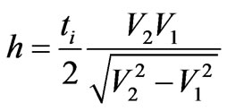 (5)
(5)
with V1 and V2 the seismic wave velocity of each layer determined from the reciprocal of the slope of the linear segments of the curve (Figure 9) and ti the intercept time. A similar equation applies to a three-layer case where three linear segments are observed in the travel-time curve.
Because the subsurface geology is rarely horizontal, a completely different approach, the delay-time method, can be used to determine variable relief on the contact of the refracting layer. This method requires data from both forward and reverse seismic lines by placing the geophone at each end of the line, and collecting data from identical shot points for each geophone location. Figure 10 gives the geometrical arrangement showing the forward and reverse paths for a given source location. It can be shown [5] that the delay-time at point C, TC, is related to the depth to the refracting surface directly below C by the expression
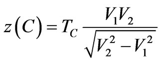 (6)
(6)
The subsurface profile is determined through calculation of z at successive locations. The value of TC can be determined by the simple expression
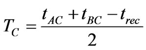 (7)
(7)
where tAC and tBC are the times required for the seismic wave to travel from the source at C to the geophones at A and B respectively ([5] p. 123). Only waves that travel
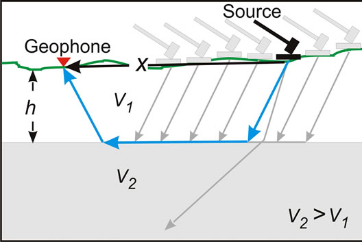
Figure 8. Illustration of the propagation of shock waves at the ground surface (black line) and subsurface (blue line) for a layered case with velocity in the upper layer V1 less than V2 the velocity of the shock wave in the lower layer. The wave that refracts at the critical angle will eventually propagate back to the surface and be detected by the geophone. For the inexpensive instrument the geophone is fixed and the source moves repeatedly.
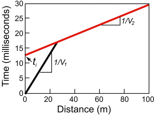
Figure 9. Typical Travel-Time curve from a seismic refraction survey. Velocities of the surface (black line) and subsurface (red line) layers (V1 and V2) can be determined from the inverse of the slopes. The intercept time, ti, together with the velocities can be used to determine the depth to the subsurface layer if the layer is horizontal.
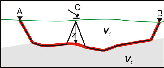
Figure 10. Illustration of the shock wave propagation for the Delay-Time method. The path for the reciprocal time is indicated in red. The depth z can be determined below each sledge hammer location to give the subsurface relief.
along the lower layer for part of their path can be used in Equation (7). The reciprocal time, trec, is the travel time from A to B. From geometrical considerations trec for a wave going from A to B must equal the time for the wave to go from B to A. It is therefore possible to determine TC at each intermediate shot point between A and B. All that is needed to determine the actual depth, z, are V1 and V2. V1 is found immediately from the travel-time curve. Burger et al. ([5] p. 124) show that V2 can be determined from the slope of the line defined by
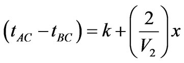 (8)
(8)
where x is the distance from A to C and k is a constant.
Although the delay-time method offers a simple means of determining subsurface relief, a much more accurate but complex procedure uses the delay time profile initially but modifies it through ray tracing until the observations are fit [12]. This procedure is coded in FORTRAN as public domain software SIPT developed by the United States Geological Survey. We developed free Windows software to make execution of SIPT more user friendly.
3.2. Construction
The design goal is to construct a reliable, easily transported seismic device for less than $250. A seismic refraction survey requires three important items: seismic source, geophone, and a seismograph. For shallow surveys a sledgehammer striking a 1-inch thick aluminum plate is usually an adequate source. A geophone is a transducer that converts slight vertical ground motion into a voltage signal. Usually this is accomplished through suspending a magnet from a spring within a coil of wire. Another approach is to use a MEMS accelerometer integrated circuit chip, which is much cheaper and smaller than a mechanical geophone and can be implemented in the same manner. Initial experiments suggest these chips have adequate sensitivity, but for the seismic survey in Chad a used geophone was purchased for $40. The seismograph records the voltage change through time, and must be able to record this signal with millisecond accuracy so that the time of first arrival of the seismic wave at the geophone can be determined. If a laptop computer is available an analog to digital converter manufactured by Measurement Computing (Personal Measurement Device “PMD”) can be used to transfer the signal to the computer through its USB port. The PMD-1208LS model can convert analog voltages into a 12-bit digital signal at a rate of 8000 samples/sec. A computer code, written in Visual Basic Net using Measurement Computing subroutines, displays the waveform on a laptop computer and permits the operator to determine elapsed time between impact of the seismic source and arrival of the first seismic wave at the geophone (Figure 11). Timing of the record must begin when the sledgehammer first strikes the plate. Upon contact, wires attached to both the plate and the sledgehammer complete an electric circuit, triggering the A/D converter. The voltage signal generated by the geophone is very small so it must be amplified before input into the PMD. A simple op-amp differential amplifier circuit which provides variable gain up to 200× (Figure 12) is adequate. The PMD must be configured properly to per-
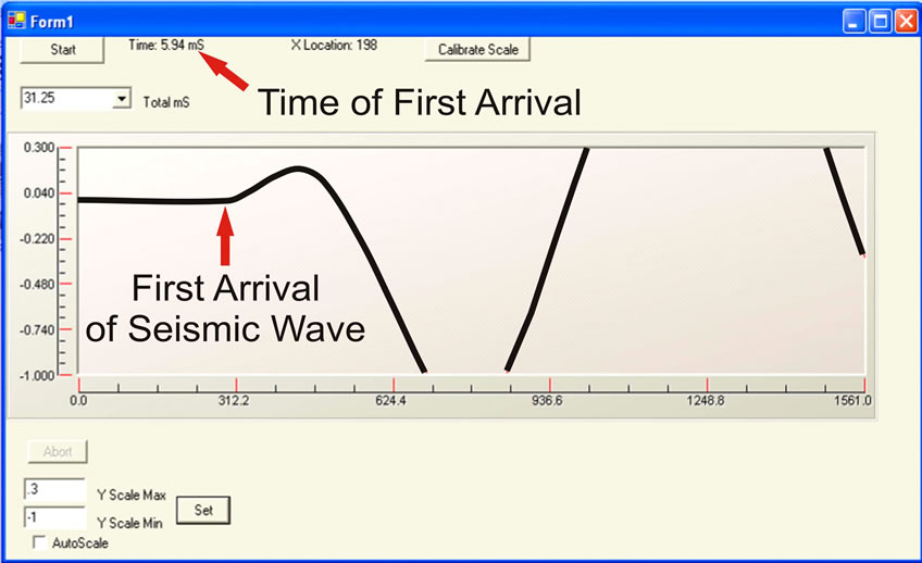
Figure 11. Laptop screen capture of a seismic wave from the PMD1208-LS Visual Basic program. The time of arrival of the first wave for known distance between the sledge and the geophone is the data required for the analysis.
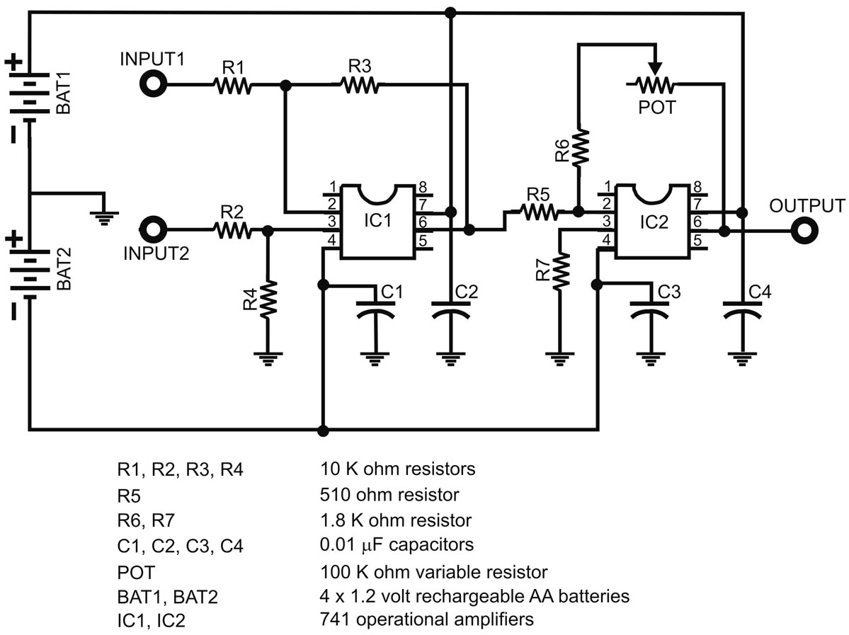
Figure 12. Electronic schematic for amplification of the seismic signal.
mit triggering, which requires a few jumper wires and a 1000 ohm resistor (Figure 13). To power or recharge a laptop a small inverter, such as the one used for a resistivity survey, should be included in the equipment list. A 60 m tape measure is also required. The instrument and geophone are shown in Figure 14. The approximate cost of each item is in Table 3 and the $245 total cost is within the design budget.
3.3. Field Method
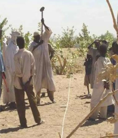
Two workers are required to conduct a seismic survey. Once a possible well site is selected, insert the geophone into the ground. If there is wind, burying the geophone a few inches greatly decreases noise and enhances the signal. Plug the geophone wires into the amplifier circuit, the trigger wires from the sledgehammer into the PMD, and then plug the PMD into the USB port of the laptop (Figure 15). Extend a tape measure about 40 m from the geophone with the tape origin at the geophone. If forward and reverse surveys are desired it is most convenient to have a constant interval for the source locations or to insert small surveying flags at each location. Launch the free seismic data collection program on the laptop and strike the plate with a mighty sledgehammer blow. It is good to involve the local people as seismic “sources” (Figure 16) because there is often healthy competition to see who can create the largest shock wave. Upon completion of the forward seismic line repeat the method for the reverse seismic line. Move the geophone to the other end of the line and bury it at the exact location of the last
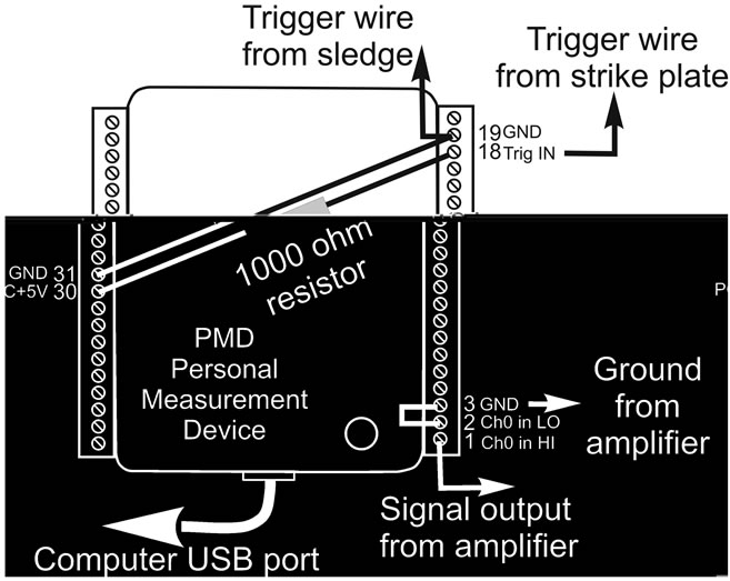
Figure 13. Electrical hookup of the Measurement Computing “Personal Measurement Device” (PMD) 1208LS.
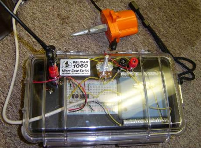
Figure 14. Instrument and geophone.
shot. As a simple check, the arrival time for the most distant point for the forward seismic line should equal the arrival time for the distant point in the reverse direc-
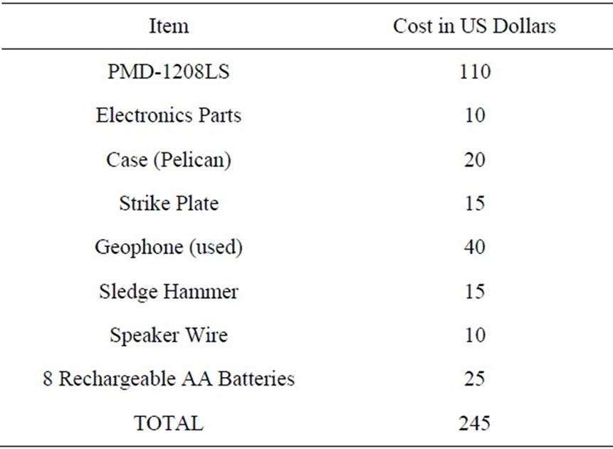
Table 3. Itemized list of seismograph materials and cost.
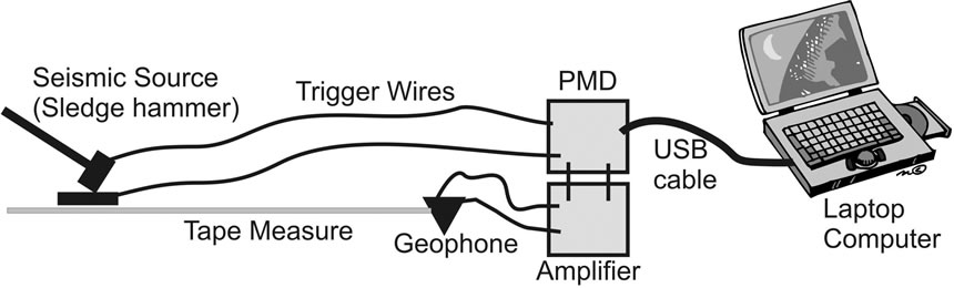
Figure 15. Schematic of field setup.
 (a)
(a)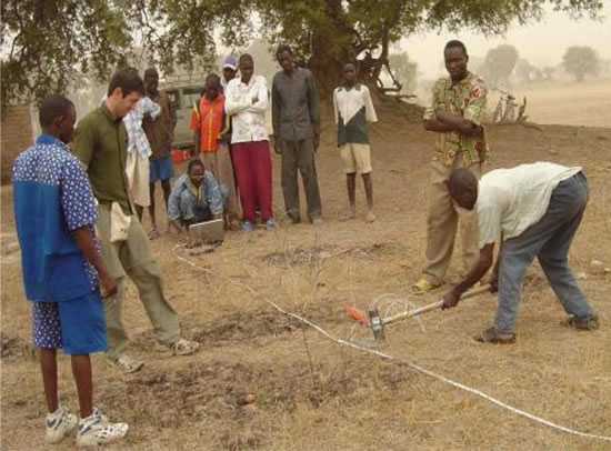 (b)
(b)
Figure 16. Use of the instrument in Chad. Local residents provided the seismic source power at Faguire (a) and Berkoman (b).
tion. This is the reciprocal time, trec, used in Equation (7). The calculations for depth and velocity can be done on a laptop in the field using our free version of the SIPT software. Output is a seismic section showing a profile of the subsurface lithologies.
3.4. Data and Results
To check the accuracy of the inexpensive seismograph, data collected with the inexpensive instrument were compared to data from an EG & G SmartSeis 12 Channel seismograph. The data from the inexpensive instrument compares favorably with the data from the $15,000 SmartSeis seismograph. The differences of only 0.4 m in depth determination (Figure 17) can easily be due to errors in assigning the time of the first arrival of the seismic wave.
The equipment was first used in Chad at the Faguire site, where the three segments in the travel-time curve (Figure 18) indicated three subsurface layers with velocities of 373, 1202 and 5356 m/sec. It was known that dry sand is the surface material and, from nearby outcrops, it was evident that granite is the bedrock at depth. Referring to Table 2 the surface velocity of 373 m/s is exactly what would be expected for dry sand and 5356 m/s is appropriate for solid granite. The intermediate layer, with a velocity of 1202 m/s could be saturated sand, but it is more likely that this is a weathered granite layer, because the existing well reached rock close to the surface. The thickness of the upper layer (Equation (5)) is then 3.4 m and the thickness of the intermediate layer is 6.4 m, so the total depth to solid granite is expected to
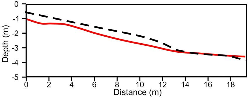
Figure 17. Comparison of the subsurface profile for the inexpensive device (solid red line) to the EG & G SmartSeis 12-channel seismograph (dashed black line). The WindowsSIPTwater program was used to calculate each profile.
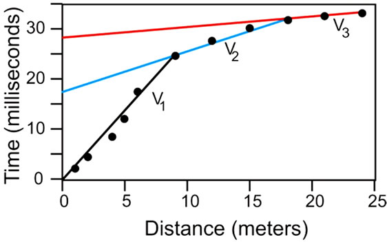
Figure 18. Indication of three layers at Faguire in a traveltime plot. Each successive change in slope represents another layer.
be 9.8 m.
At Berkoman in southwestern Chad both forward and reverse seismic lines were completed. The data shown in the travel-time plot (Figure 19) indicate a 2-layer earth. Some scatter about the lines suggests that the dipping contact has some subtle relief. These data were used in our modified SIPT program to produce a seismic section (Figure 20). Where the time-delay method is used, the predicted curve shows depth to the contact between the upper sediment (374 m/s velocity) and the underlying substrate (1796 m/s). When the ray tracing algorithm is included using SIPT the contact depth is only slightly changed and smoothed.
3.5. Discussion
The inexpensive seismograph is accurate and capable of detecting shallow strata under developing world conditions. In addition to the huge cost savings, this instrument is very small, light, and portable. The sledge hammer has the greatest bulk and mass. All but the sledge can be packed into a small suitcase. The modified SIPT software (called WindowsSIPTwater.exe) provides excellent interpretations of subsurface relief and is readily used while in the field. Although the instrument was tested where layers are shallow, it would be ideal to penetrate at least 20 m, which would typically require a spread about 80 m long. A stronger seismic source such as an explosive or a “Betsy gun” shotgun source would be required, but would certainly be out of the question in the developing world. Transporting explosives on aircraft would also be problematic. A solution is to stack sledge hammer blows so that a weak signal is added to previous signals, enhancing the signal while simultaneously canceling any random noise. This stacking ability is now included in our seismic recording software. Another feature common on commercial units is the ability to filter certain frequencies. The physical properties of the geophone do this to some extent, and this feature is needed less for refraction surveying than for reflection surveying. An improvement to the device would be a simple active low cut or high cut filter.
Two workers can measure and record each seismic signal in 3 to 4 minutes. A seismic survey with 12 shot locations would take about 1.5 hours to complete, since both forward and reverse lines are needed. Importing the data and running WindowsSIPTwater takes about 30 minutes.
The problems that can arise with seismic refraction are clearly described in most texts. The most important assumption is that deeper strata must have progressively higher velocities. For example where low velocity sediment (e.g. sand) underlies a higher velocity layer (e.g.
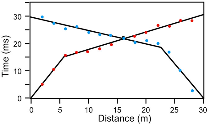
Figure 19. Travel-Time data at Berkoman, Chad. The forward (red data points) and reverse (blue data points) surveys are not symmetrical indicating the subsurface layer is tilted.
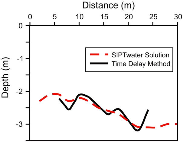
Figure 20. Comparison of the Time-Delay method to the ray tracing method of WindowsSIPTwater at Berkomann, Chad.
well-packed clay) the seismic wave refracts downward, not upward, and the sand will be invisible in the interpretation. Very thin layers may not be observed.
4. Final Discussion
The indigenous men and women who we trained were eager to learn the methods and quick to apply them. Some may argue that extensive training is necessary to insure interpretation errors are avoided, which would be true if elaborate instruments are used or highly varied geology is encountered. More likely these inexpensive instruments will be used in localized regions by drillers and aid workers who will not travel great distances. In Tanzania the geologic stratigraphy consists of clay overlying bedrock and in Chad sand or silt overlies bedrock with depth the only unknown. Once a geophysical survey is finished the well that is subsequently drilled will provide excellent ground truth to compare to predictions. Such comparisons will undoubtedly lead to revisions and improvement of future geophysical interpretations in the region.
The seismic refraction method requires a laptop computer, and interpretation of earth resistivity is greatly aided with one. It is the laptop that is most likely to fail under field conditions. Fortunately even the cheapest of modern laptops has ample CPU and storage capacity to execute the software needed for the surveys. Acceptable laptop computers are now available for less than $400. Furthermore the computer can perform other useful tasks in support of drilling. For example, the free OpenOffice suite provides spreadsheet, word processing and presentation capability useful in report preparation. QuantumGIS is a public domain Geographic Information System (GIS) with good remote sensing capability in its GRASS module. Satellite images are often free and can be used with GIS to search for natural fracture trends, lineaments or moist regions [16]. An inexpensive GPS (i.e. less than $120) can be used to record well locations for input into the GIS as well as for navigation. If a geophysical team travels first and records the locations of good well sites, then a GPS will allow accurate re-establishment of the sites for subsequent drilling. In Tanzania original survey locations recorded with GPS by government geologists were successfully re-established by us within 2 meters.
Finally, free groundwater models, such as PMWIN, can give insight into groundwater flow in a region and the effects of well pumping in low yield areas. A laptop computer may serve many useful purposes in support of groundwater exploration, so its expense is readily justified.
The suite of geophysical resistivity and seismic refraction instruments including a laptop computer can be assembled for less than $850, the cost of a hand auger. More than half of that cost is the laptop, which can be used for much more than just geophysical surveys.
5. Conclusions
With the cost so reasonable (less than $850) this equipment should become common among those desiring to provide water in developing countries. The instruments are small, light, robust, inexpensive and easy to construct. With the free software available the interpretation of data is not difficult, although care still is needed. The free software described in this paper can be downloaded from http://cs.wheaton.edu/~jclark.
6. Acknowledgements
We wish to thank the Wheaton College Alumni Association for support both in the development of the resistivity device and for funding the field work. St. Paul Partners paid for drilling the wells, materials used in the resistivity meter, salaries of the Tanzanian drilling team, and general logistics within Tanzania. Keith Olson led the LifeWater International team and greatly encouraged the development of the instruments. It is to his memory that this paper is dedicated. The Evangelical Lutheran Church of Tanzania and Rev. Lambert Mtatifikolo provided much needed support while in Tanzania. Christy Page assisted with the Tanzanian field work and Daniel Clark helped in the development of the resistivity instrument. Dr. Phil Carpenter helped test the resistivity device.
We also wish to thank the Timothy Project, a Senior Scholarship Achievement Award from Wheaton College and the Wheaton College Alumni Association Gieser Award for funds in support of the seismic work. Pastor Ngarndeye Bako, Director of Entente des Eglises Et Missions Evangeliques au Tchad (EEMET) in Chad, provided advice, hospitality, and friendship. Sambim Kosdonlengar (EEMET), Stephen Moss (Wheaton College) and Tanya Thomas (World Relief) provided essential help during all phases of the field work. The EEMET and the United Nations High Commission on Refugees (UNHCR) provided travel while in Chad. Chris Gregory tested the seismograph with the EG&G SmartSeis instrument. We would especially like to thank Don Church for his encouragement in promoting all phases of these projects. Publication of this paper was possible through funds provided by Will Chester and Emma Sarbu at the time of their marriage engagement. May their life together be God glorifying.
REFERENCES
- W. M. Telford, L. P. Geldart, R. E. Sheriff and D. A. Keys, “Applied Geophysics,” Cambridge University Press, Cambridge, 1982.
- R. D. Barker, C. C. White and J. F. T. Houston, “Borehole Siting in an African Accelerated Drought Relief Project,” In: E. P. Wright and W. G. Burgess, Eds., Hydrogeology of Crystalline Basement Aquifers in Africa, Geological Society Special Publication, No. 66, 1992, pp. 183-201. doi:10.1144/GSL.SP.1992.066.01.09
- R. Kirsch (Ed.), “Groundwater Geophysics: A Tool for Hydrogeology,” Springer, New York, 2006.
- W. Rabbel, “Seismic Methods,” In: R. Kirsch, Ed., “Groundwater Geophysics: A Tool for Hydrogeology,” Springer, New York, 2006, pp. 23-83.
- H. R. Burger, A. F. Sheehan and C. H. Jones, “Introduction to Applied Geophysics: Exploring the Shallow Subsurface,” W. W. Norton & Company, New York, 2006
- R. Herman, “An Introduction to Electrical Resistivity in Geophysics,” American Journal of Physics, Vol. 69, 2001, pp. 943-952. doi:10.1119/1.1378013
- M. J. Hornbach, “Development and Implementation of a Portable Low Cost Seismic Data Acquisition System for Classroom Experiments and Independent Studies,” Journal of Geoscience Education, Vol. 52, 2004, pp. 386-390.
- J. A. Olowofela, V. O. Jolaosho and B. S. Badmus, “Measuring the Electrical Resisitivity of the Earth Using a Fabricated Resisitivity Meter,” European Journal of Physics, Vol. 26, 2005, pp. 501-515. doi:10.1088/0143-0807/26/3/015
- D. P. Ghosh, “The Application of Linear Filter Theory to the Direct Interpretation of Geoelectrical Resistivity Sounding Measurements,” Geophysical Prospecting, Vol. 19, 1971, pp. 192-217. doi:10.1111/j.1365-2478.1971.tb00593.x
- D. P. Ghosh, “Inverse Filter Coefficients for the Computation of Apparent Resistivity Standard Curves for a Horizontally Stratified Earth,” Geophysical Prospecting, Vol. 19, 1971, pp. 769-775. doi:10.1111/j.1365-2478.1971.tb00915.x
- E. Orellana and H. M. Mooney, “Master Tables and Curves for Vertical Electrical Sounding over Layered Structures,” Interciencia, Madrid, 1966.
- J. H. Scott, “SIPT—A Seismic Refraction Inverse Modeling Program for Timeshare Terminal Computer Systems,” USGS Open-File Report, 1977, pp. 77-365.
- S. H. Ward, “Resistivity and Induced Polarization Methods,” In: S. Ward, Ed., Geotechnical and Environmental Geophysics: Review and Tutorial, Vol. 1, Society of Exploration Geophysicists Investigations in Geophysics, 1990, pp. 147-189. doi:10.1190/1.9781560802785
- D. W. Steeples, “Shallow Seismic Methods,” In: Y. Rubin and S. S. Hubbard, Eds., Hydrogeophysics, Vol. 50, Part. 2, 2005, pp. 215-251. doi:10.1007/1-4020-3102-5_8
- R. H. Brown, P. A. Konoplyantsev, J. Ineson and V. S. Kovalevsky (Eds.), “Groundwater Studies: An International Guide for Research and Practice,” UNESCO Studies and Report in Hydrology, No. 7, Sect. 9.1, 1997, p. 2.
- S. Mutiti, J. Levy, C. Mutiti and N. S. Gaturu, “Assessing Ground Water Development Potential Using Landsat Imagery,” Ground Water, Vol. 48, 2010, pp. 295-305. doi:10.1111/j.1745-6584.2008.00524.x