Journal of Water Resource and Protection
Vol. 2 No. 6 (2010) , Article ID: 2071 , 9 pages DOI:10.4236/jwarp.2010.26064
Differential Evolution Algorithm with Application to Optimal Operation of Multipurpose Reservoir
1Department of Civil Engineering, Government College of Engineering,
Aurangabad, India
2Research Scholar, National Institute of Technology, Warangal, India
3Department of Civil Engineering, National Institute of Technology, Warangal, India
E-mail: {dgregulwar, sumantchoudhari}@rediffmail.com, a_raj_p@yahoo.co.in
Received March 12, 2010; revised April 7, 2010; accepted May 4, 2010
Keywords: Optimization, Hydropower Production, Differential Evolution, Reservoir Operation
ABSTRACT
This paper includes an application of Differential Evolution (DE) for the optimal operation of multipurpose reservoir. The objective of the study is to maximize the hydropower production. The constraints for the optimization problem are reservoir capacity, turbine release capacity constraints, irrigation supply demand constraints and storage continuity. For initializing population, the upper and lower bounds of decision variables are fixed. The fitness of each vector is evaluated. The mutation and recombination is performed. The control parameters, i.e., population size, crossover constant and the weight are fixed according to their fitness value. This procedure is performed for the ten different strategies of DE. Sensitivity analysis performed for ten strategies of DE suggested that, De/best/1/bin is the best strategy which gives optimal solution. The DE algorithm application is presented through Jayakwadi project stage-I, Maharashtra State, India. Genetic algorithm is utilized as a comparative approach to assess the ability of DE. The results of GA and ten DE strategies for the given parameters indicated that both the results are comparable. The model is run for dependable inflows. Monthly maximized hydropower production and irrigation releases are presented. These values will be the basis for decision maker to take decisions regarding operation policy of the reservoir. Results of application of DE model indicate that the maximized hydropower production is 30.885 × 10⁶ kwh and the corresponding irrigation release is 928.44 Mm3.
1. Introduction
Water for drinking purpose, for use in industry, irrigation and hydropower production, is main factor for hindering developments in many parts of the globe. Hence, proper management of available water resources is essential. Reservoir operation forms an important role in water resources development. Yeh [1] reviewed reservoir management and operation models. Algorithms and methods surveyed include linear programming (LP), dynamic programming (DP), nonlinear programming (NLP), and simulation. Oliveira and Loucks [2] have presented operating rules for multireservoir systems by using genetic search algorithms. Simulation was used to evaluate each policy by computing performance index for a given flow series. Wardlaw and Sharif [3] have presented several alternative formulations of a genetic algorithm for reservoir system. Later on, multi-reservoir systems optimization has been studied by Sharif and Wardlaw [4]. Nagesh Kumar et al. [5] have studied optimal reservoir operation for hydropower production which involved constrained nonlinear optimization. Earlier to that Srinivasa Raju and Nagesh Kumar [6] have discussed application of genetic algorithms for irrigation planning. GA was used to determine optimal cropping pattern for maximizing benefits for an irrigation project. Regulwar and Anand Raj [7] have presented A Multi objective, Multireservoir operation model for maximization of irrigation releases and hydropower production using Genetic Algorithm. A monthly Multi Objective Genetic Algorithm Fuzzy Optimization (MOGAFUOPT) model has been developed. From the relationships developed amongst irrigation releases, hydropower production and level of satisfaction, a three dimensional (3-D) surface covering the whole range of policies has been developed.
Storn [8] has represented a heuristic approach for minimizing nonlinear and non differentiable continuous space function. The proposed method which requires few control variables is robust, easy to use and lends itself very well to parallel computation. Lampinen [9] has proposed differential evolution algorithm for handling nonlinear constraint functions. Differential Evolution (DE) algorithms claimed to be very efficient when they are applied to solve multimodal optimal control problems (Lopez Cruz et al. [10]). Differential evolution was used for the optimization of non-convex Mixed Integer Nonlinear Programming (MINLP) problems. The results of DE were compared with simplex, simulated annealing and genetic algorithm (Babu and Angira [11]). Vasan and Srinivasaraju [12] have demonstrated application of differential evolution to Bilaspur project in Rajasthan, India. The objective was to determine suitable cropping pattern for maximum benefits. Ranjithan [13] has presented the role of evolutionary computation in environmental and water resources systems analysis and discussed various methods such as Simulated Annealing, Tabu Search, GA, Evolutionary strategies, Particle swarm and Ant colony optimization. Janga Reddy and Nagesh Kumar [14] have studied Multi Objective Differential Evolution (MODE) with an application to a reservoir system optimization. The evolutionary operators used in differential evolution algorithms are very much suitable for problems having interdependence among the decision variables.Vasan and Komaragiri Srinivasa Raju [15] have demonstrated the applicability of DE to a case study of Mahi Bajaj Sagar project (MBSP), India. Ten different strategies of DE were employed to assess the ability of DE for solving higher dimensional problems as an alternative methodology for irrigation planning. The results were compared with LP.
In Genetic Algorithm (GA) low mutation rate is required to get global optimum [16]. The low mutation rate may get trouble with problems having interdependent relationships between variables and may require more number of function evaluations [17]. In reservoir operation the interdependence relationship may exist among decision variables. Interdependencies among variables can be tackled by properly rotating the co-ordinate system of the given function as it is done in Differential Evolution. DE has all properties necessary to handle complex problems with interdependencies between parameters [18]. DE maintains correlated self-adopting mutation step sizes in order to make timely progressive optimization. There is interdependence among variables therefore the evolutionary operators of DE are suitable to tackle these problems. This paper presents the applicability of DE for determining operation policies of a multipurpose reservoir.
2. Methodology
Differential evolution is a recent evolutionary optimization technique. It is simple, faster convergent and robust. The main difference between GA and DE is that GA depends on crossover while DE uses mutation as primary search mechanism. DE uses weighted differences between solution vectors to perturb the population. Unlike genetic algorithms, no binary coding of the population members is necessary. The general convention used for different variants of DE is DE/a/b/c. Here DE is for Differential evolution, ‘a’ is a string which denotes the vector to be perturbed, ‘b’ denotes the number of difference vectors taken for perturbation of ‘a’ and ‘c’ is the crossover method. According to Price and Storn [19] different strategies of DE are DE/rand/1/bin, DE/best/1/bin, DE/ best/2/bin, DE/rand/2/bin, DE/rand-to-best/1/bin, DE/ rand/1/exp, DE/best/1/exp, DE/best/2/exp, DE/rand/2/ exp, and DE/rand-to-best/1/exp.
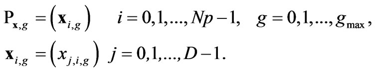
DE holds D-dimensional real valued vectors of Np population in pair. The current population Px, includes vectors xi,g added or created randomly or by comparison with other vectors.
 (1)
(1)
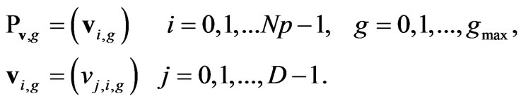
The index, g = 0, 1,… gmax, shows the generation of a vector. A population index i is assigned to each vector which ranges from 0 to Np-1. The index ‘j’ indicates parameter within vector ranges from 0 to D-1. After initialization, an intermediary population Pv,g, of Np mutant vectors, vi,g produced by random mutation.
 (2)
(2)
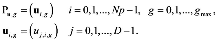
Each vector in the current population is then recombined with a mutant to produce a trial population, Pu of Np trial vectors, ui,g
 (3)
(3)
During crossover, trial vectors overwrite the mutant population, so a single array can hold both populations. Then the cost of the trial vector is compared with the cost of the target vector, the vector having low cost will go into the next generation.
2.1. Case Study
The Jayakwadi project stage-I is taken as a case study. It is built across river Godavari, in Maharashtra State, India. The gross storage of reservoir is 2909 ´ 106 m3 and live storage is 2171 ´ 106 m3. Total installed capacity for power generation is 12.0 MW (Pumped storage plant). Irrigable command area is 1416.40 km2. The schematic representation of the physical system showing Jayakwadi project stage-I is shown in Figure 1. Monthly historical flow data for 73 years is collected and 75% dependable monthly flows are estimated using the Weibull plotting position formula. The inflow, irrigation demand, turbine capacity are presented in Table 1.
2.2. Model Formulation
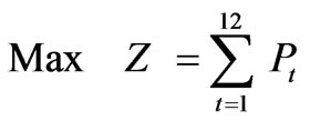
The objective of the study is to maximize the hydropower production and present operation policy of a case study reservoir. Mathematically it can be expressed as:
 (4)
(4)
where Pt = Hydropower produced in kwh during month ‘t’. If the monthly releases for hydropower (RP) are
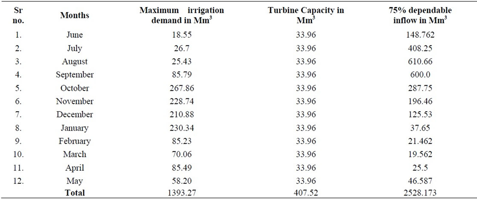
Table 1. Inflow, irrigation demand and power demand.
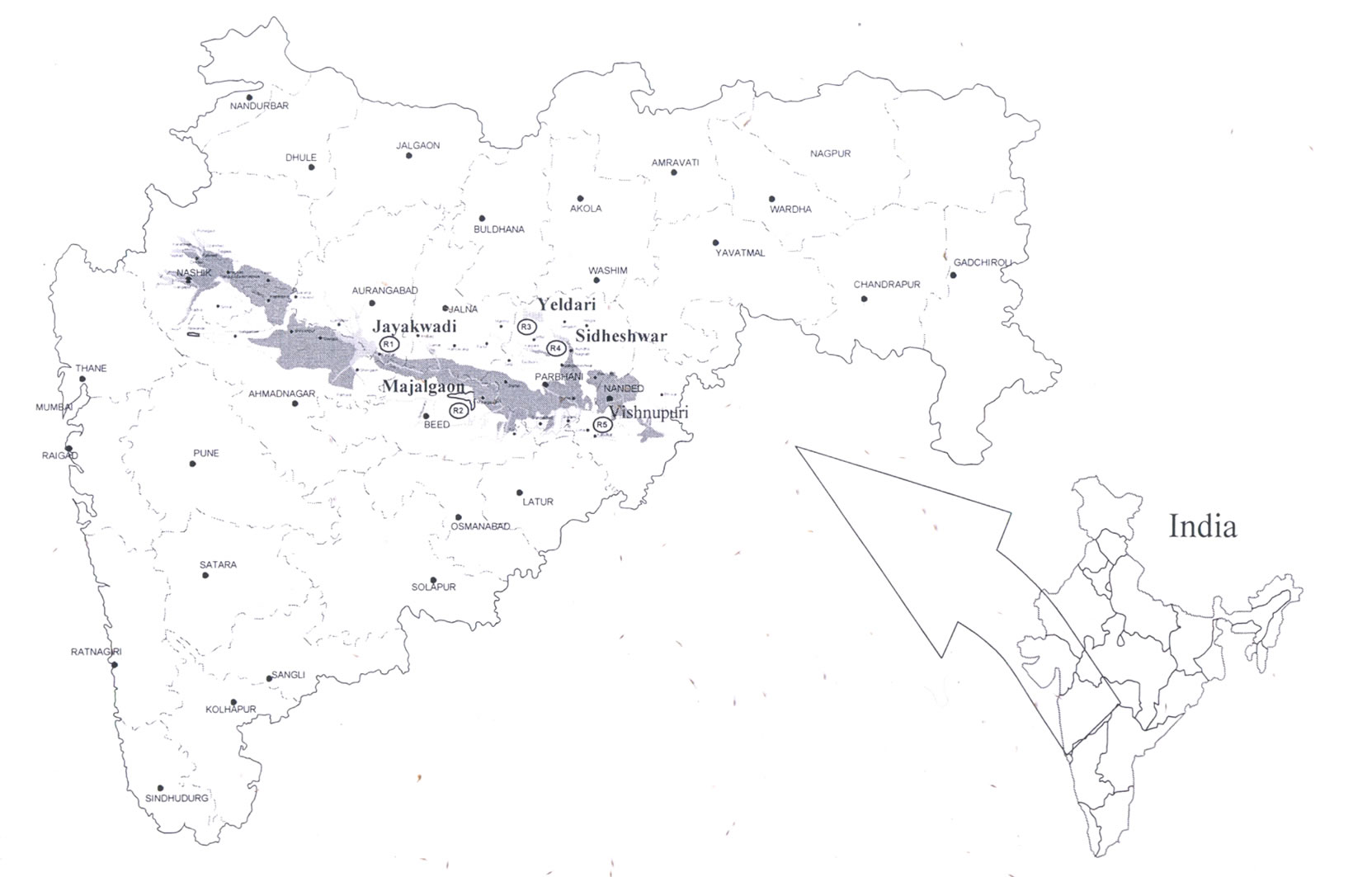
Figure 1. Sketch showing Jayakwadi project stage-1, Maharashtra state, India.
expressed in Mm3, head (h) in meters, then power produced P in KW hours for a 30 day month is given by P = 2725 × (RP) × (h). The model is subjected to the following constraints.
2.2.1. Releases into Turbine and Capacity Constraints
The releases into turbines for power production, should be less than or equal to the flow through turbine capacity (TC) for all the months. Also, power production in each month should be greater than or equal to the firm power (FP). These constraints can be written as:
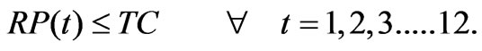 (5)
(5)
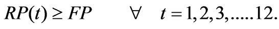 (6)
(6)
2.2.2. Irrigation Supply-Demand Constraints
The releases into canals for irrigation (RI) should be less than or equal to the maximum irrigation demand (IDmax) for all the months. Also, the releases into the canals for irrigation should be greater than or equal to the minimum irrigation demand (IDmin). The irrigation release-demand constraint, can, therefore be written as:
 (7)
(7)
 (8)
(8)
2.2.3. Reservoir Storage-Capacity Constraints
The storage in the reservoirs (S) should be less than or equal to the maximum storage capacity (SC) and greater than or equal to the minimum storage capacity (Smin) for all months. These constraints can be written as:
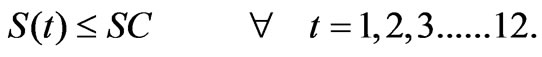 (9)
(9)
 (10)
(10)
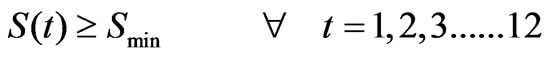
2.2.4. Reservoir Storage-Continuity Constraints
This constraint relate to the turbine releases (RP), irrigation releases (RI), release for drinking and industrial water supply (RWS) which is taken as a constant, reservoir storage (S), inflows into the reservoirs (IN), Losses from the reservoirs for all months. The losses from the reservoirs are taken as function of storage as given by Loucks et al. [20]. Let Ao is reservoir water surface area corresponding to the dead storage volume and et is evaporation rate corresponding to the time period t (in depth units). Aa is the reservoir water spread area per unit volume of active storage. Then the actual evaporation during the time period ‘t’ is given by
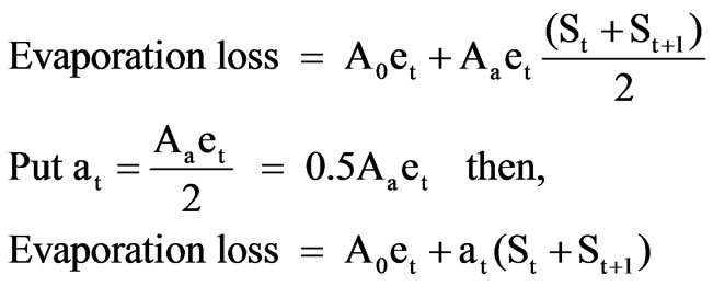
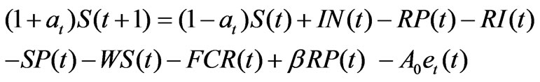
Then the hydrologic continuity constraint can be written as:
 (11)
(11)
3. Results and Discussion
Differential Evolution (DE) has ten strategies. The model is run with DE parameters, i.e., crossover constant and weight for each strategy. The population is fixed by running the model for different population sizes in combination with crossover constants and weight. For deciding crossover constant and weight for each strategy, the model is run for different crossover constants, i.e., 0.7, 0.75, 0.8, 0.85, 0.9, 0.95 with the combination of weight ranging from 0.2 to 0.9 with the increment of 0.05. For every combination fitness is calculated and compared with population. Based on this approach population is fixed as 400. For getting optimal solution, generation is fixed as 500. The DE parameters, i.e., crossover constants and weight are decided for each strategy and presented in Table 2. The relationships between weight and hydropower releases corresponding to crossover constant are presented graphically in Figures 2 to 11. By considering these DE parameters, the optimization model is run and optimized values of objective function are presented for all strategies in Table 2. The random seed should be greater than one. So for seed also the model is run for various seed values, i.e., 1 to 90, and 77 is fixed from the comparison of results.
Table 2 presents comparison of strategies of DE. In this table, the crossover constant, weight, optimal hydropower production and annual irrigation releases are presented corresponding to each strategy. The comparison of strategies for maximum objective function value is shown graphically in Figure 12. From the Table 2, it is clear that the strategy number 6, i.e., DE/best/1/bin gives the optimal results. For this strategy, the DE parameters are crossover 0.85, and weight 0.9. The optimized hydropower production is worked out to be 30.89 × 10⁶ kwh. The release for irrigation corresponding to the optimal fitness of objective function is 928.44 Mm3. Monthly optimal releases for irrigation are shown graphically in Figure 13. Monthly optimal hydropower production is shown graphically in Figure 14. For comparison of DE results, the genetic algorithm approach is utilized in this study. The proposed reservoir operation model is solved using GA. Stochastic remainder selection; one point crossover and binary mutation are used as GA operators in this study. For selection of population size, crossover probability, mutation probability and optimal generations, a thorough sensitivity analysis is carried out. The system performance is estimated by taking crossover probability between 0.6 to 1.0 with a increment of 0.05 and mutation probabilities between 0.4 to 0.001 with a decrement of 0.1 up to 0.01 and then the decrement is taken as 0.001. The population size is var-
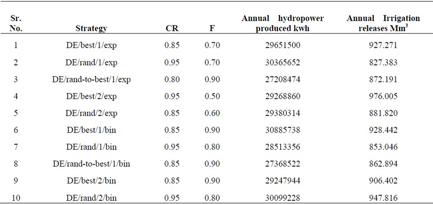
Table 2. Comparison of strategies of differential evolution.
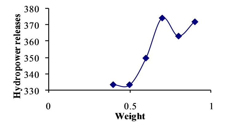
Figure 2. Relationship between weight and strategy No. 1 for crossover 0.85.
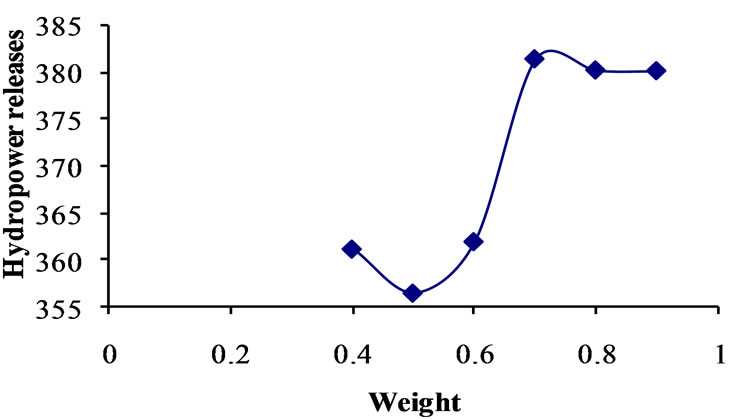
Figure 3. Relationship between weight and strategy 2 for crossover 0.95.
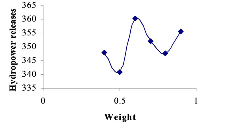
Figure 4. Relationship between weight and strategy No. 3 for crossover 0.8.
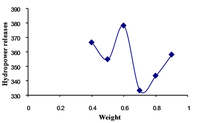
Figure 5. Relationship between weight and strategy No. 4 for crossover 0.95.
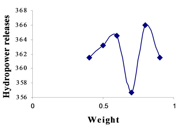
Figure 6. Relationship between weight and strategy No. 5 for crossover 0.85.
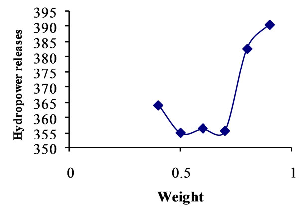
Figure 7. Relationship between weight and strategy No. 6 for crossover 0.85.
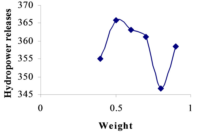
Figure 8. Relationship beween weight and strategy No. 7 for crossover 0.95.
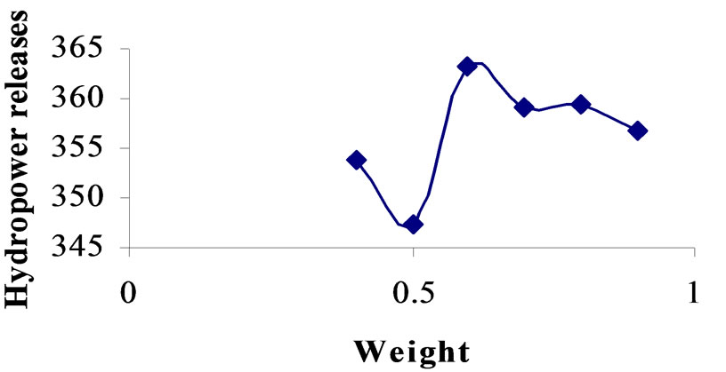
Figure 9. Relationship between weight and strategy No. 8 for crossover 0.85.
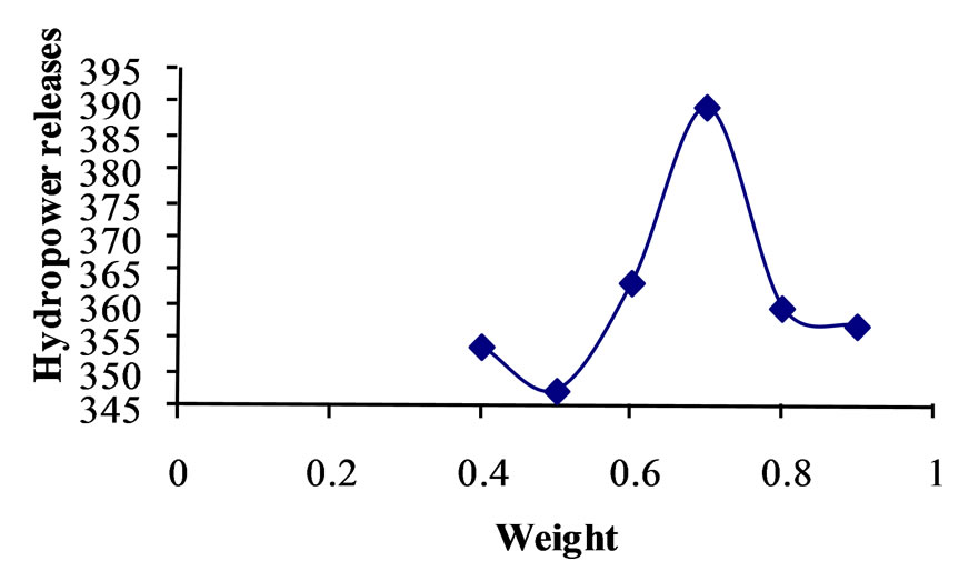
Figure 10. Relationship between weight and strategy No. 9 for crossover 0.85.
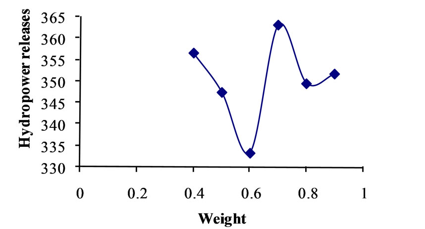
Figure 11. Relationship between weight and strategy No. 10 for crossover 0.95.
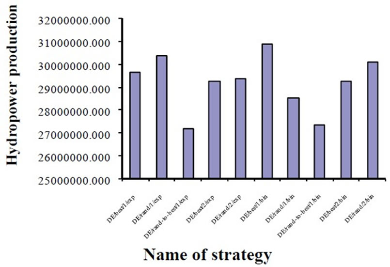
Figure 12. Comparison of strategies.
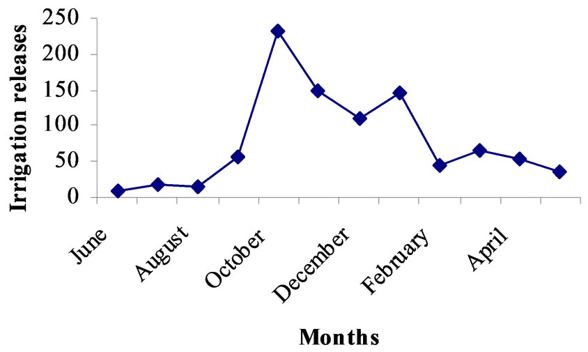
Figure 13. Optimal releases for irrigation (DE/best/1/bin).
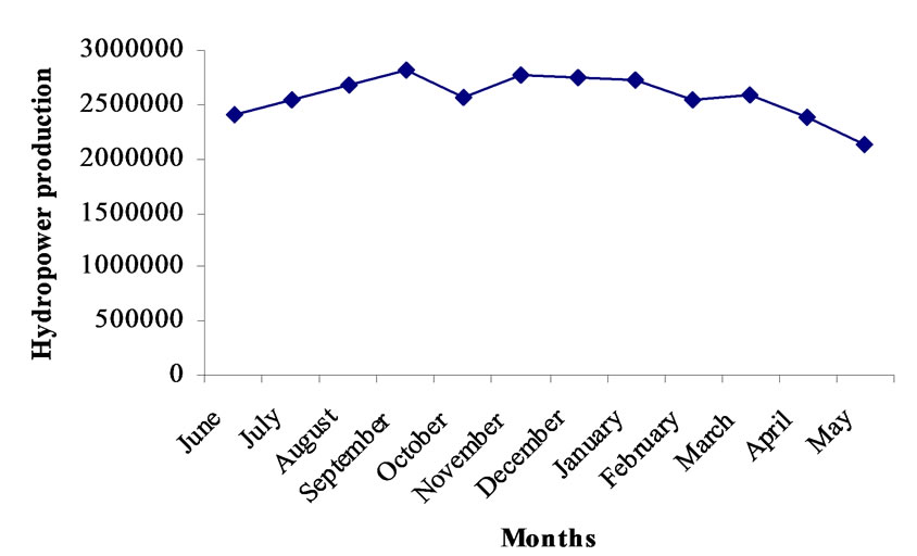
Figure 14. Optimal hydropower production (DE/best/1/bin).
ied from 50 to 150 and generation from 20 to 500. Based on the system performance the optimal population size and optimal number of generations are 100 and 500 respectively. For crossover probability of 0.95 and mutation probability of 0.01, the maximization is achieved. The monthly optimized irrigation releases and hydropower production by using GA are obtained and presented in Table 3. The comparison of DE and GA results for irrigation releases and hydropower production are presented for best strategy in the same table. Also Table 4 represents the monthly optimal irrigation releases obtained by DE strategies and GA. Table 5 represents the
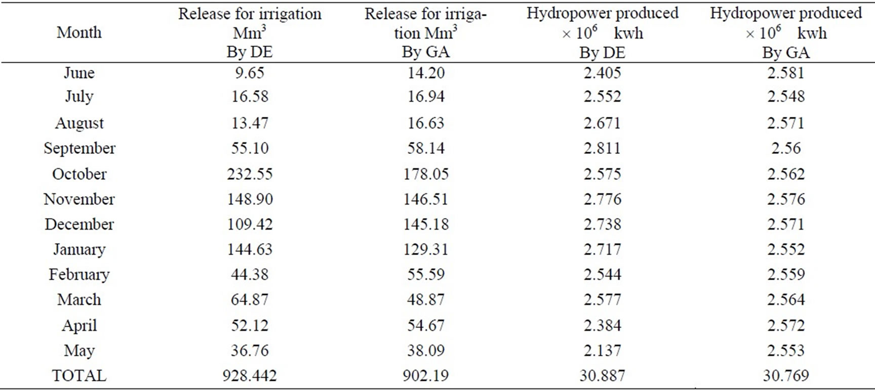
Table 3. Comparison of optimal releases for irrigation and hydropower production by DE and GA.
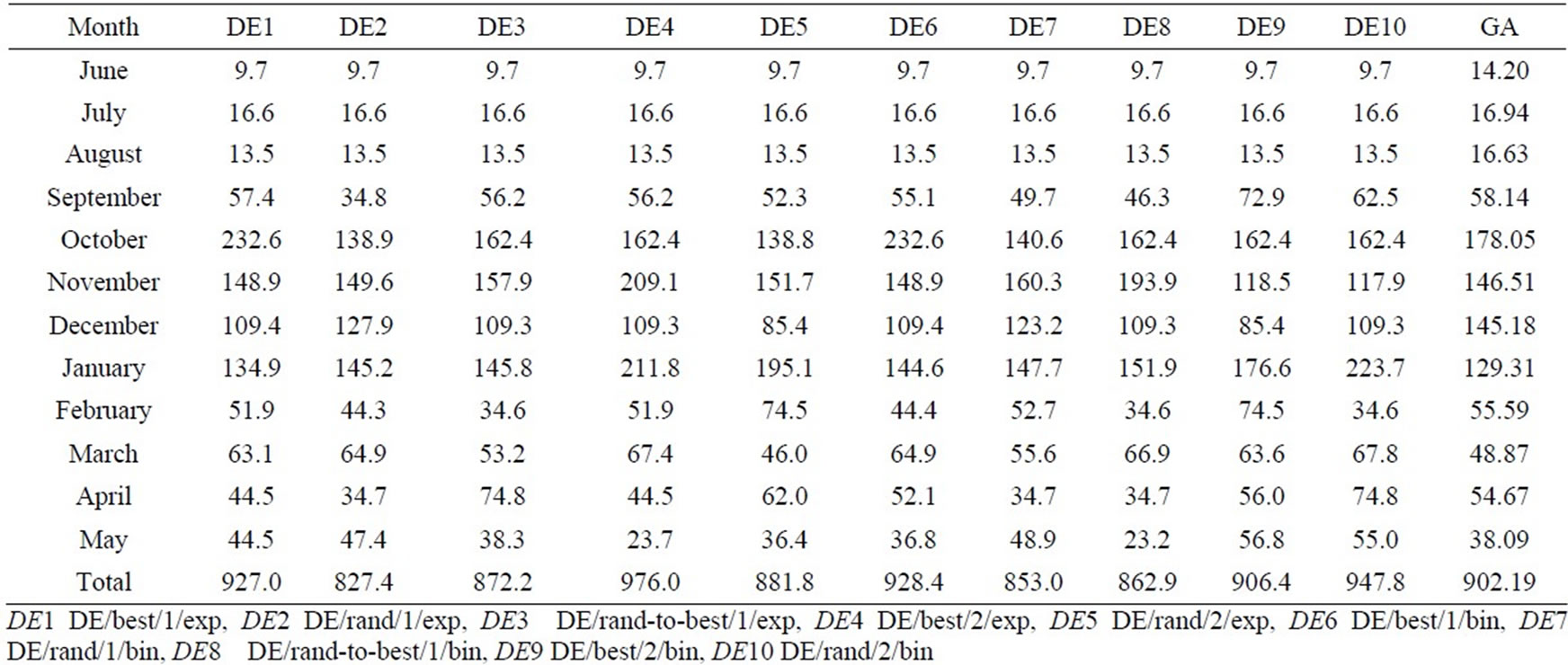
Table 4. Irrigation releases obtained by the DE strategies and GA in Mm3.
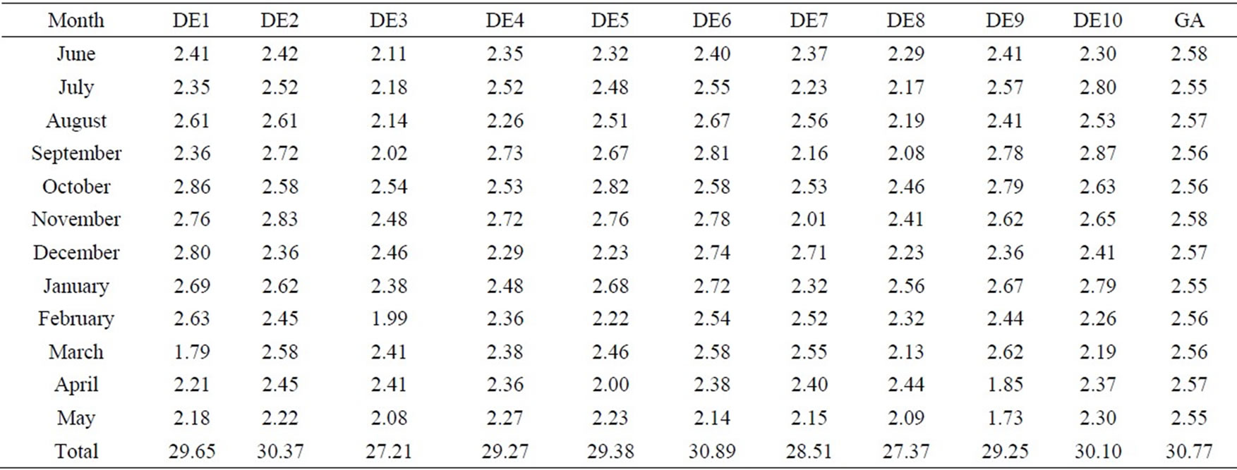
Table 5. Hydropower production obtained by the DE strategies and GA in kwh (× 106).
monthly optimal hydropower production by DE strategies and GA. Tables 4 and 5 gives exhaustive comparison of all DE strategies and GA for irrigation releases and hydropower production. This comparison among all strategies of DE and GA provides applicability of differential evolution for optimal operation of multi-purpose reservoir.
4. Conclusions
In the present study a multipurpose reservoir in Godavari River sub basin in Maharashtra State, India is considered. A multiobjective operation model for maximization of hydropower production is proposed using differential evolution algorithm. Results of application of DE model indicate that the maximized hydropower production is 30.885 × 10⁶ kwh and the corresponding irrigation release is 928.44 Mm3. From the results it can be seen that the monthly maximized irrigation release and hydropower production can be the basis for decision maker to take decision for reservoir operation. Genetic algorithm is utilized as a comparative approach. The results of GA and different DE strategies for irrigation releases and hydropower production show that both the results are close and comparable. Therefore it can be said that DE can be used as an alternative methodology for optimal operation of multipurpose reservoir. Differential evolution algorithm works with numerical values. Therefore highly complex objective functions do not introduce any difficulties and even discontinuous functions are acceptable. From the results, it can be said that the DE can be effectively applied to multi-objective operation problem and the reservoir can be operated for optimal reservoir releases for irrigation and hydropower production after meeting the other demands from the reservoir.
5. Acknowledgements
The authors are thankful to Rainer Storn, K. Price and J. Lampinen for their guidance during the work. Also, the authors are thankful to Command Area Development Authority, Aurangabad, Maharashtra state, India for providing necessary data for the analysis.
REFERENCES
- W. W.-G. Yeh, “Reservoir Management and Operations Models: A State-of-the-Art Review,” Water Resources Research, Vol. 21, No. 12, 1985, pp. 1797-1818.
- R. Oliveira and D. P. Loucks, “Operating Rules for Multi-Reservoir Systems,” Water Resource Research, Vol. 33, No. 4, 1997, pp. 839-852.
- R. Wardlaw and M. Sharif, “Evaluation of Genetic Algorithm for Optimal Reservoir System Operation,” Journal of Water Resource, Planning and Management, Vol. 125, No. 1, 1999, pp. 25-33.
- M. Sharif and R. Wardlaw, “Multireservoir Systems Optimization Using Genetic Algorithms: Case Study,” Journal of Computer in Civil Engineering, Vol. 14, No. 4, 2000, pp. 255-263.
- D. Nagesh kumar, A. Kumar and K. S. Raju, “Application of Genetic Algorithms for Optimal Reservoir Operation,” Proceedings of X World Water Congress, Melbourne, 2000.
- K. S. Raju and D. Nagesh Kumar, “Irrigation Planning Using Genetic Algorithms,” Water Resource Management, Vol. 18, No. 2, 2004, pp. 163-176.
- D. G. Regulwar and P. A. Raj, “Development of 3-D Optimal Surface for Operation Policies of a Multireservoir in Fuzzy Environment Using Genetic Algorithm for River Basin Development and Management,” Water Resource and Management, Vol. 22, No. 5, 2008, pp. 595- 610.
- R. Storn and K. Price, “Differential Evolution a Simple Evolution Strategy for Fast Optimization,” Dr Dobb’s Journal, Vol. 22, No. 4, 1997, pp. 18-24.
- J. Lampinen, “Multiconstraint Nonlinear Optimization by Differential Evolution Algorithm,” Technical Report, Lappeenranta University of Technology, Laboratory of Processing, 1999. http://www.lut.fi/~jlampine/debiblo.htm
- I. L. Lopez Cruz, L. G. Van Willigenburg and G. Van Straten, “Efficient Differential Evolution Algorithms for Multimodal Optimal Control Problems,” Journal of Applied Soft Computing, Vol. 3, No. 2, 2003, pp.97-122.
- B. V. Babu and R. Angira, “A Differential Evolution Approach for Global Optimization of MINLP Problems,” Proceedings of 4th Asia Pasific conference on Simulated Evolution and Learning (SEAL2002), Vol. 2, Singapore, 2002, pp. 880-884.
- A. Vasan and K. Srinivasa Raju, “Optimal Reservoir Operation Using Differential Evolution,” International Conference on Hydraulic Engineering: Research and Practice (ICON-HERP-2004), Indian Institute of Technology Roorkee, India, 2004.
- S. R. Ranjithan, “Role of Evolutionary Computation in Environmental and Water Resources Systems Analysis,” Journal of Water Resources Planning and Management, ASCE, Vol. 131, No. 1, 2005, pp.1-2.
- M. J. Reddy and D. N. Kumar, “Multiobjective Differential Evolution with Application to Reservoir System Optimization,” Journal of Computing in Civil Engineering, ASCE, Vol. 21, No. 2, 2007, pp.136-146.
- A. Vasan and K. S. Raju, “Application of Differential Evolution for Irrigation Planning: An Indian Case Study,” Water Resources Management, Vol. 21, No. 8, 2007, pp. 1393-1407.
- D. E. Goldberg, “Genetic Algorithms in Search, Optimization and Machine Learning,” Addison-Wesley, Reading, Massachusetts, 1989.
- R. Salomon, “Re-Evaluating Genetic Algorithm Performance under Coordinate Rotation of Benchmark Functions: A Survey of Some Theoretical and Practical Aspects of Genetic Algorithms,” Biology Systems, Vol. 39, No. 3, 1996, pp. 263-278.
- K. V. Price, “An Introduction to Differential Evolution, New Ideas in Optimization,” McGraw-Hill, London, 1999, pp. 79-108.
- K. Price and R. Storn, “Home Page of Differential Evolution,” 2005. http://www.icsi.Berkeley.edu/~storn/code.html
- D. P. Loucks, J. Stedinger and D. Haith, “Water Resources Systems Planning and Analysis,” Prentice-Hall, Eaglewood Cliffs, New Jersey, 1981.
Appendix: Notation
The following symbols are used in this paper
RP(t): Monthly releases for power generation during month t
TC: Flow corresponding to maximum capacity of turbine
FP: Flow corresponding to firm power.
RI(t): Releases for irrigation during month t.
IDmax(t): Maximum irrigation requirement of command area during month t.
IDmin (t): Minimum irrigation requirement of command area during month t
S(t): Storage volume in the reservoir during month t
SC: Maximum storage volume of reservoir
Smin: Dead storage volume of reservoir
SP(t): Spills during month t
FCR(t): Feeder Canal Releases during month t
β: Constant.
NP: Number of Population
CR: Crossover Constant
F: Weight