Journal of Biomedical Science and Engineering
Vol.6 No.1(2013), Article ID:27444,9 pages DOI:10.4236/jbise.2013.61008
A new method of analysing the intracerebral haemorrhage signal intensity on brain MRI images using frequency domain techniques
![]()
1Electronics and Communication Engineering, Gogte Institute of Technology, Belgaum, India
2Vishwanathrao Deshpande Rural Institute of Technology, Haliyal, India
3Indian Institute of Technology (Madras), Belgaum, India
4RAGAVS, Diagnostics and Research Center Pvt Ltd., Bangalore, India
Email: supriya_sp@yahoo.com
Received 12 November 2012; revised 18 December 2012; accepted 25 December 2012
Keywords: Diffusion Images; High Frequency Power; Intracerebral Haemorrhage; Magnetic Resonance Imaging; Signal Intensity
ABSTRACT
Diffusion Weighted Magnetic Resonance Imaging (DW-MRI) has become an established part of neuroimaging and is used to diagnose and characterize several neurologic disorders. Intracerebral Haemorrhage (ICH) is a severe medical condition, which may develop quickly into a life-threatening situation, and thereby requires prompt medical attention. Early and reliable identification of the age of haemorrhage is essential when choosing the correct treatment, and estimating patient’s diagnosis and outcome. Diffusion Weighted (DW) images presents a variation in the image signal intensity characteristics relative to the different stages of ICH. In the present paper, an effort is made to document the variation in the image signal intensity characteristics of ICH at evolving stages, for 30 subjects, using High Frequency Power (HFP) parameter. Results showed that the difference in the HFP values on DW images for the subjects with ICH compared to their contralateral normal hemisphere, were highly significant (p < 0.01) in areas of the brain, where there was a high incidence of ICH. The relative increase in the image signal intensity HFP values (RHFP) for the subjects with ICH were in the range of (31.0 - 2477.32) times compared to their corresponding HFP values on the contralateral normal hemisphere. The observed RHFP values were elevated in Stage 1 (Hyperacute: <1 day) of ICH and further progressively decreased in Stage 2 (Acute: 1 - 7 days) and Stage 3 (Late subacute: 7 - 14 days), and eventually reached their minimum in Stage 4 (Chronic: >14 days). There was a negative correlation (r = −0.81) observed between the RHFP values and the evolving stages of ICH. The results indicate that the quantitative changes in the RHFP values can be assessed to derive information about the stage of ICH, and their adoption in clinical diagnosis and treatment could be helpful and informative.
1. INTRODUCTION
Intracerebral Haemorrhage (ICH) is a potentially lifethreatening medical emergency of the highest degree, which often causes early neurological deterioration. ICH is responsible for up to 15% of all strokes and is associated with a high rate of mortality [1]. Patients with ICH face an increased risk of death and long term functional disability, compared to other forms of stroke, even for lesions of similar size or location [2]. This results in huge demand on health care resources and has thereby driven research and investigations in this area. Diagnosis of ICH involves neuroimaging options, and Computed Tomography (CT) has traditionally been used in radiologic workup of ICH. However, numerous studies have demonstrated that Magnetic Resonance Imaging (MRI) is more efficient in detecting ICH and in localizing ICH [3-5]. The development of ICH on conventional MRI is well described and documented in literature [6-10]. Studies indicate that the appearance of ICH on MRI primarily depends on the stage of haemorrhage and on the imaging sequence or parameters. Investigators have reported high diagnostic accuracy of MRI for ICH within a time window of 2.5 to 5 hours after symptom onset [11]. In spite of the frequent use of conventional MRI to assess the appearance of ICH over the past few years, Diffusion Weighted Magnetic Resonance Imaging (DW-MRI) has only recently been accepted as a valuable investigative resource. DW-MRI has changed the overall importance of imaging in the clinical setting by providing unique information on the viability of brain tissue and consequently on patient management. This sequence produces MRI based quantitative maps of microscopic, natural displacements of water molecules that occur in brain tissues as part of the physical diffusion process [12,13]. Water molecules are used as probes that reveal microscopic details about the architecture of both healthy and unhealthy brain tissues [14]. The generalized model for the appearance of ICH on Magnetic Resonance (MR) images attributes the various signal intensity patterns of evolving ICH, to the oxygenation state of hemoglobin and the integrity of the red blood cells [6,15]. Correspondingly the signal intensity characteristics on DW images of the brain undergo a series of variations after the onset of ICH, that can be instructive in identifying the stage of ICH.
Several studies have been carried out to characterize haemorrhage on the basis of DW-MRI findings, and they qualitatively indicate that hematomas are initially hyper-intense on Diffusion Weighted (DW) images and later hypo-intense during the first few days after onset [15-18]. Other investigators have recognized that hematoma signal intensity on DW images varies with time [19], but have not thoroughly quantified these signal intensity changes. Furthermore there are reports that describe the temporal evolution of Apparent Diffusion Coefficient (ADC) values within lesions following ICH, to identify their usefulness in clinical diagnosis of ICH and treatment [15,19-22].
For subjects with ICH, early and reliable estimation of ICH stage is of importance, since it shows the exact state of brain injury and the state of inflammation. This information further affects the rest of the therapy. It is generally observed that the radiologists in a variety of clinical settings depend on the signal intensity variations on DW images to quickly assess subjects with ICH [15,18,19, 23], wherein, the hematoma signal intensity is visually graded as hyper-, iso-, or hypo-intense, relative to the normal contralateral hemisphere. Such a procedure requires high level of expertise in this field considering the complex parameters that affect the appearance of ICH on DW images. Thereby such estimation by observation method is to some extent sensitive to experience and may be subjected to misunderstanding of the actual stage of ICH. Thus, if the progression of the image signal intensity on DW images following ICH can be automatically quantified and assessed, this information would surely aid the radiologists in early and accurate diagnosis of the stage of ICH. This would result in subjects receiving prompt treatment, thereby protecting them from any further damage to the brain tissue.
The purpose of the present work is to measure the clinical utility of DW-MRI in the diagnosis and treatment of subjects with ICH, with the hope to improve patient outcome. In this direction we have analyzed the evolution of image signal intensity on DW images of the human brain in the axial plane, to identify the different levels of changes taking place in the subjects with ICH. Mainly an effort is made to grade the image signal intensity variations on DW images, using High Frequency Power (HFP) values, for subjects with ICH, compared to their corresponding HFP values obtained from the contralateral normal hemisphere. The ADC methods reported in literature to study the signal characteristics of ICH on DW images, at evolving stages, rely on a single axial section (showing ICH) to carry out observations. Also the calculation of ADC values considers only a small region within the area of haemorrhage. This would need a thorough understanding of the entire haemorrhagic area for accurate analysis, as the ADC values vary within the area of haemorrhage [18]. In contrast, the present work takes into account all the axial sections that show ICH on DW images, and further considers the entire area of the haemorrhage on each axial section, to evaluate the image signal intensity HFP values.
Therefore the present method simplifies the estimation process and assures that there is no loss of information, as it covers larger area of the brain. Also expertise is not essential as the entire area of the haemorrhage is taken into account for investigation. Overall, the main advantage of the proposed method is that the quantitative changes in the image signal intensity HFP values obtained from DW images can be assessed, and can most likely aid in identifying the stages of ICH, as accurate identification of ICH stage is a critical step in planning the appropriate therapy.
2. MATERIALS AND METHODS
Studies carried out in the past suggest that diffusion is restricted in the area of haemorrhage before and after cell lysis, resulting in bright signal intensity on DW images [15,19]. Further, studies show that the appearance of signal intensities on DW images transforms from being hyper-intense to hypo-intense as the haemorrhage evolves with time, from one stage to another [15,18,19]. Therefore it is very essential in understanding the characteristic features of the signal intensity variations on DW images post haemorrhage, as it can be supportive in both characterization and differentiation of the various stages of ICH. Accordingly, detection of the areas of brain with high signal intensity variations on DW images, subsequent to ICH, may allow for the evaluation of the affected area. Further, quantification of the observed signal intensity may prove to be useful in the early diagnosis, characterization and proper planning of the clinical treatment for ICH.
2.1. Clinical Data and MR Imaging
The retrospective study of MR examinations in the present work was performed on 30 patients (22 male, 08 female, ages ranging from 28 years to 85 years with an average age of 55 years) with ICH unrelated to infarction. The appearance of ICH for all the 30 subjects was confirmed by ruling out the possibility of bright signal on DW images that is not due to restricted diffusion, but rather due to high T2 signal which “shines through” to the DW image, referred to as T2 shine through. This was done by verifying the appearance of hyper-intensities on DW images and concomitant reduced ADCs relative to the contralateral normal brain in their initial MRI studies. Further all the subjects showed magnetic susceptibility artifact on gradient echo sequence, confirming it is haemorrhage. The ethics approval was obtained from the committee of clinical research at the RAGAVS Diagnostic and Research center, Bangalore, India, and Vikram Hospital, Bangalore, India.
The evolution of ICH can be described by five distinct stages, namely Hyperacute (<1 day), Acute (1 - 3 days), Early subacute (3 - 7 days), Late subacute (7 - 14 days) and Chronic (>14 days) [6,9]. However Acute and Early subacute stages of ICH display similar appearance on DW images [19,24]. For this reason, in the present work we have grouped the Acute and Early subacute stages of ICH collectively to form Stage 2, that is, the Acute stage (1 - 7 days). MR studies undertaken at various intervals after the onset of symptoms, defined four stages of ICH according to the duration of the interval between the onset and initial MR examination. The four stages were: Stage 1: Hyperacute (five subjects within 24 hours of symptom onset); Stage 2: Acute (six subjects between days 1 and 7); Stage 3: Late subacute (twelve subjects between days 7 and 14) and Stage 4: Chronic (seven subjects after 14 days).
All the subjects underwent clinical MR imaging with 1.5 T symphony maestro class MR scanning system from Siemens. DW imaging was performed by using a multisection, single-shot, spin-echo, echo-planar pulse sequence with following parameters: Repetition Time [TR] = 3200 ms, Echo Time [TE] = 94 ms, acquisition matrix = 128 × 128, Field of View [FOV] = 230 mm × 230 mm, and diffusion gradient value of b = 1000 s/m2 along 19 axial sections, 5 mm thick section and intersection gap of 1.5 mm.
2.2. Image Signal Intensity High Frequency Power
DW-MRI technique makes it to visualize the altered rates of water diffusion, by producing a bright imaging appearance in the area of ICH when compared to the normal tissues, at different stages of ICH. Consequently on examining the spatial intensity variation distribution on DW images for the subjects with ICH, it is observed that the image signal intensity is not uniformly distributed over the entire DW image, and marks sudden changes in the area of haemorrhage, when compared to the other normal areas of the brain. The spatial intensity characteristics of an image can be related to the frequency components of the Fourier transform, since frequency is directly related to rate of change of intensity variations in an image. Low frequencies correspond to slowly varying components and high frequencies correspond to faster varying components, such as abrupt change in the image intensity levels [25]. Exploring the power spectrum of the DW intensity image for the subject with ICH would thereby result in a higher value for the higher spatial frequency power component, out of the total power spectrum, in the area of haemorrhage, when compared to the higher spatial frequency power component on the contralateral normal (healthy) hemisphere (mirror image) of the same subject [25]. In the present work an attempt is made to analyze DW images for the subjects with ICH in the frequency domain, using image signal intensity HFP parameter. HFP component in the total power spectrum in the area of haemorrhage is compared to the corresponding HFP component obtained from the contralateral normal hemisphere. The relative image signal intensity HFP (RHFP) values are quantified across different subjects diagnosed with ICH, using Eq.1 (see below).
The RHFP values so obtained are employed in differentiating the haemorrhage tissues from healthy tissues, and further used in the categorization of the different stages of ICH. The obtained RHFP values could possibly aid neuro-surgeons for immediate diagnosis and execution of treatment, by providing information about the stage of ICH.
2.3. Image Analysis
DW images obtained in DICOM format are converted to bmp format with intensities scaled to fit the conventional range of (0 - 255). This is done to reduce the complexity in the image manipulation algorithms, and to achieve speed up in processing the images. DW image obtained from each subject in the axial plane is divided into six anatomically significant areas as shown in Figure 1.
For each subject with ICH, we obtain a set of DW images in the axial plane taken at different axial sections (from 1 to 19). The subject with ICH presents abrupt
 (1)
(1)
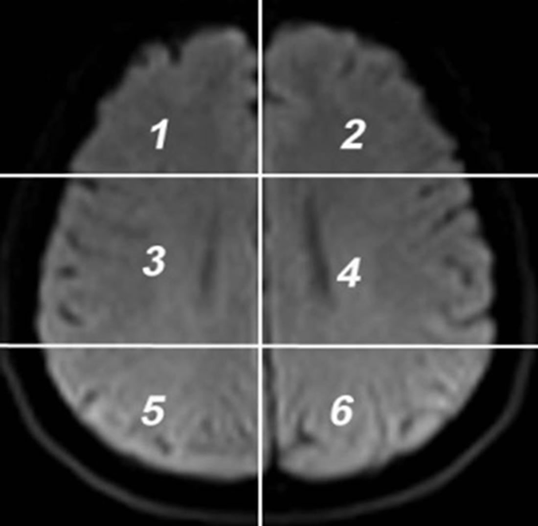
Figure 1. Axial DW image showing areas.
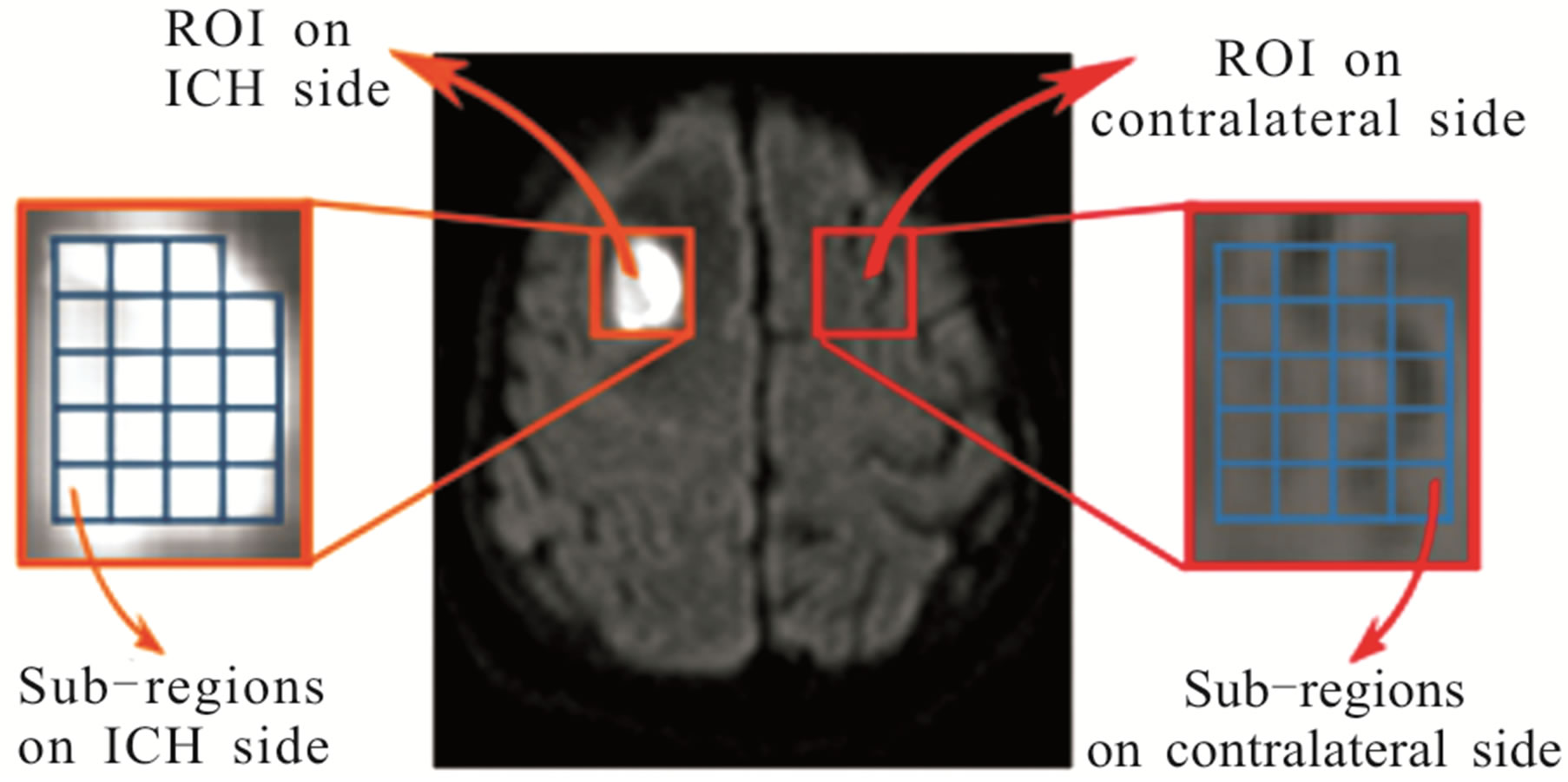
changes in the image signal intensity in one (or more) of the six areas, in the affected axial sections. The axial sections that indicate such abrupt changes in the image signal intensities are selected for image analysis. For each axial section selected from the ICH subject, the following procedure is employed to obtain a decisive image signal intensity HFP value for that subject. Firstly a Region of Interest (ROI), I(x, y), is manually placed in the particular area of DW image, covering the high intensity region showing ICH, for that axial section. An equivalent (mirror) ROI of the same size is manually selected on the contralateral normal hemisphere of the same subject for comparison [26]. The ROIs on each side are further divided automatically (using Adobe Photoshop CS3) into smaller sub-regions, f(x, y), corresponding to an image size represented by (M × N) pixels. The typical values for M and N selected for image analysis range in between 15 to 18 pixels. Additional care is taken while choosing the sub-regions to avoid any errors that may be caused due to edge effects (change in intensity along the periphery of ICH). The ROI and the corresponding sub-regions on the ICH side and on the contralateral normal hemisphere for a subject with ICH (area 1, axial section 16) are shown in Figure 2(a). The image intensity distribution for a particular sub-region on the ICH side and the corresponding sub-region on the contralateral normal hemisphere is shown in Figures 2(b) and (c) respectively. The Fourier spectrum, F(u, v), of an image, f(x, y), corresponding to a sub-region of the ROI is evaluated. The spatial frequencies and their distribution for these sub-regions are analysed by performing the two-dimensional Discrete Fourier Transform (DFT) using MATLAB version 7.7.
The spatial frequencies (u and v) are denoted by cycles per pixel, since the image size (distance) for the analysis is given in terms of pixels. Using the periodicity property of DFT [25], the Fourier spectrum is shifted to the center of the frequency plane. The DC component, F(0, 0), is deleted, since it gives only the average value of the image intensity. The power spectrum is obtained by squar-
 (a)
(a)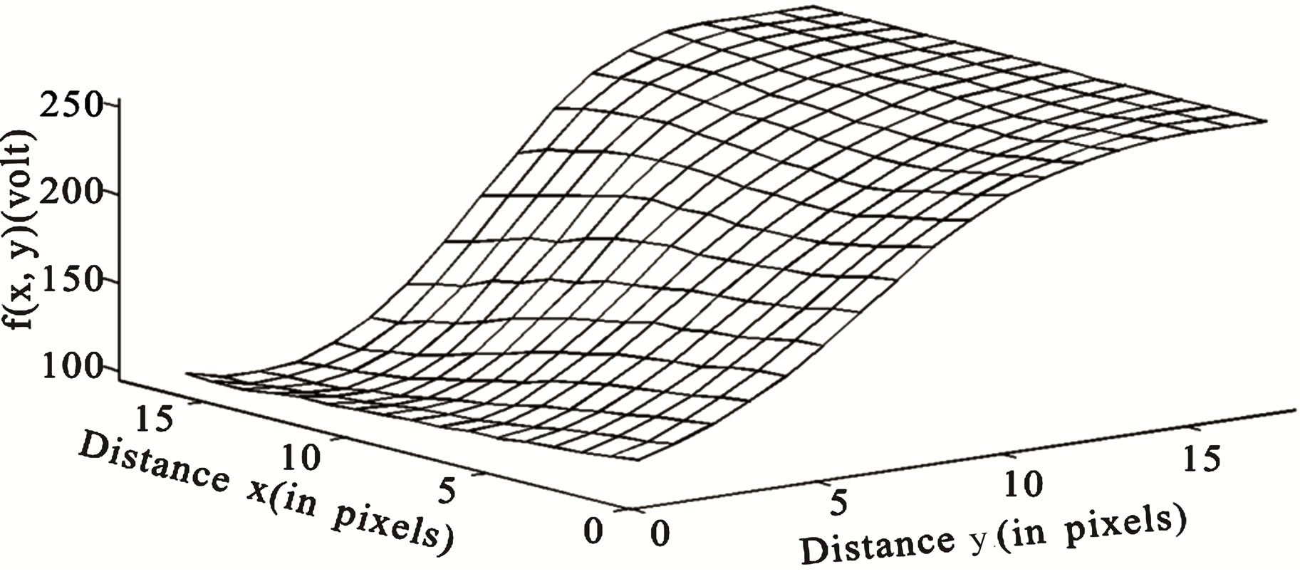 (b)
(b)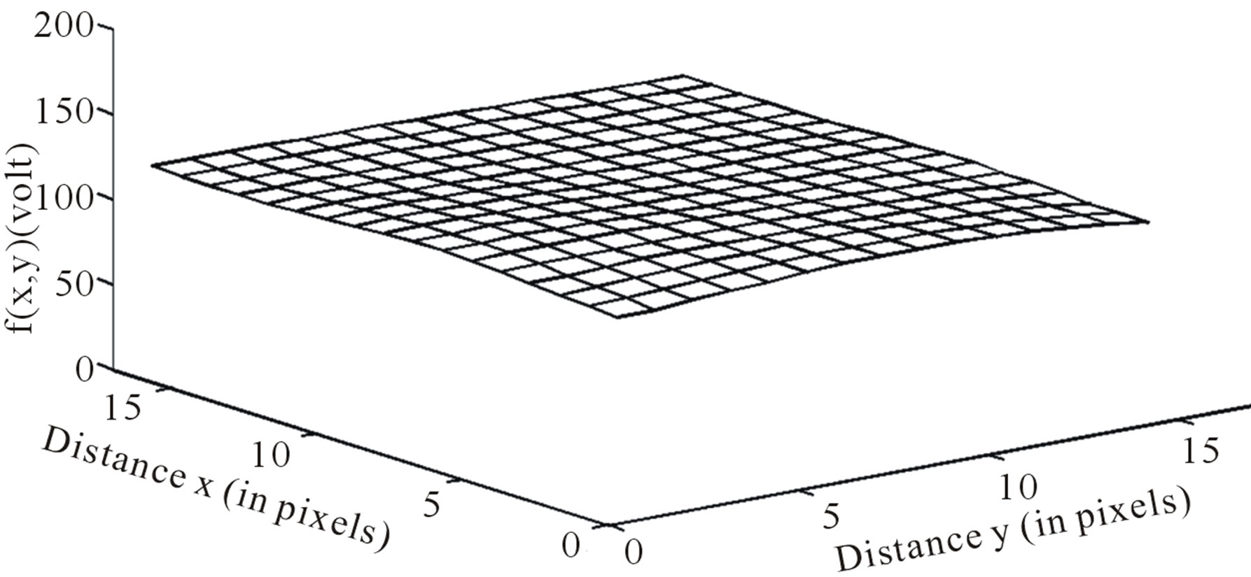 (c)
(c)
Figure 2. (a) Axial DW image showing ROI (I(x, y)) and sub-regions (f(x, y)) on ICH side (area 1, axial section 16) and contralateral side (b) Image intensity distribution for a subregion (18 pixels × 17 pixels) on ICH side (c) Image intensity distribution for corresponding sub-region (18 pixels × 17 pixels) on contralateral normal side.
ing the magnitudes of the Fourier spectrum image signal intensity variations [25,27] of DW image and the Total Power (TP), in the image is obtained using Eq.2.
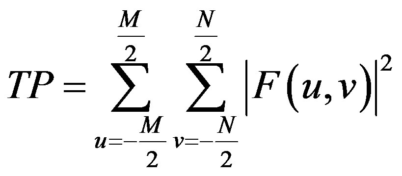 (2)
(2)
Since for the sub-regions of the brain, the values of M and N are different (depend on the size of the particular sub-region), the cut-off frequency, D0 (in cycles per pixel), which separates the lower and higher spatial frequency components (as shown in Figure 3), is defined by Eq.3.
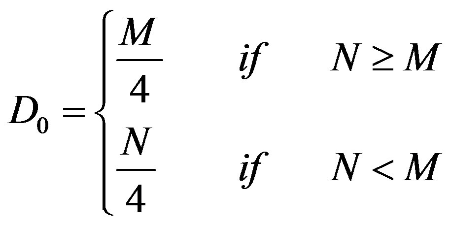 (3)
(3)
where D(u, v) is the distance from the point (u, v) to the origin of the frequency plane, defined by Eq.4.
 (4)
(4)
The value of the cut-off frequency, D0, has been decided as per the publications of other investigators [27,28]. The Low Frequency Power (LFP) and HFP are calculated using Eqs.5 and 6 respectively.
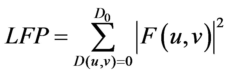 (5)
(5)
 (6)
(6)
For each sub-region on the ICH side and the corresponding sub-region on the contralateral normal side, the magnitude and the location of the image signal intensity HFP value is evaluated. Subsequently, the value of the maximum image signal intensity HFP over the entire ROI, for that axial section, on the ICH side is obtained. The corresponding image signal intensity HFP value from the contralateral normal hemisphere is noted for comparison. The magnitude of the maximum image signal intensity HFP value so obtained indicates whether there is any sudden change in the signal intensity level, in any of the sub-regions of the ROI for that axial section, for the ICH subject. Further if there is any such change observed, we can readily establish the sub-region, and also the exact location ((x, y) coordinates) within that sub-region.
The process is repeated for all the axial sections selected for image analysis from the ICH subject. After obtaining the maximum image signal intensity HFP values for all the axial sections, the value of overall maximum HFP across all the selected axial sections, is chosen as the decisive image signal intensity HFP value for that ICH subject. The equivalent image signal intensity HFP value from the contralateral normal hemisphere is noted
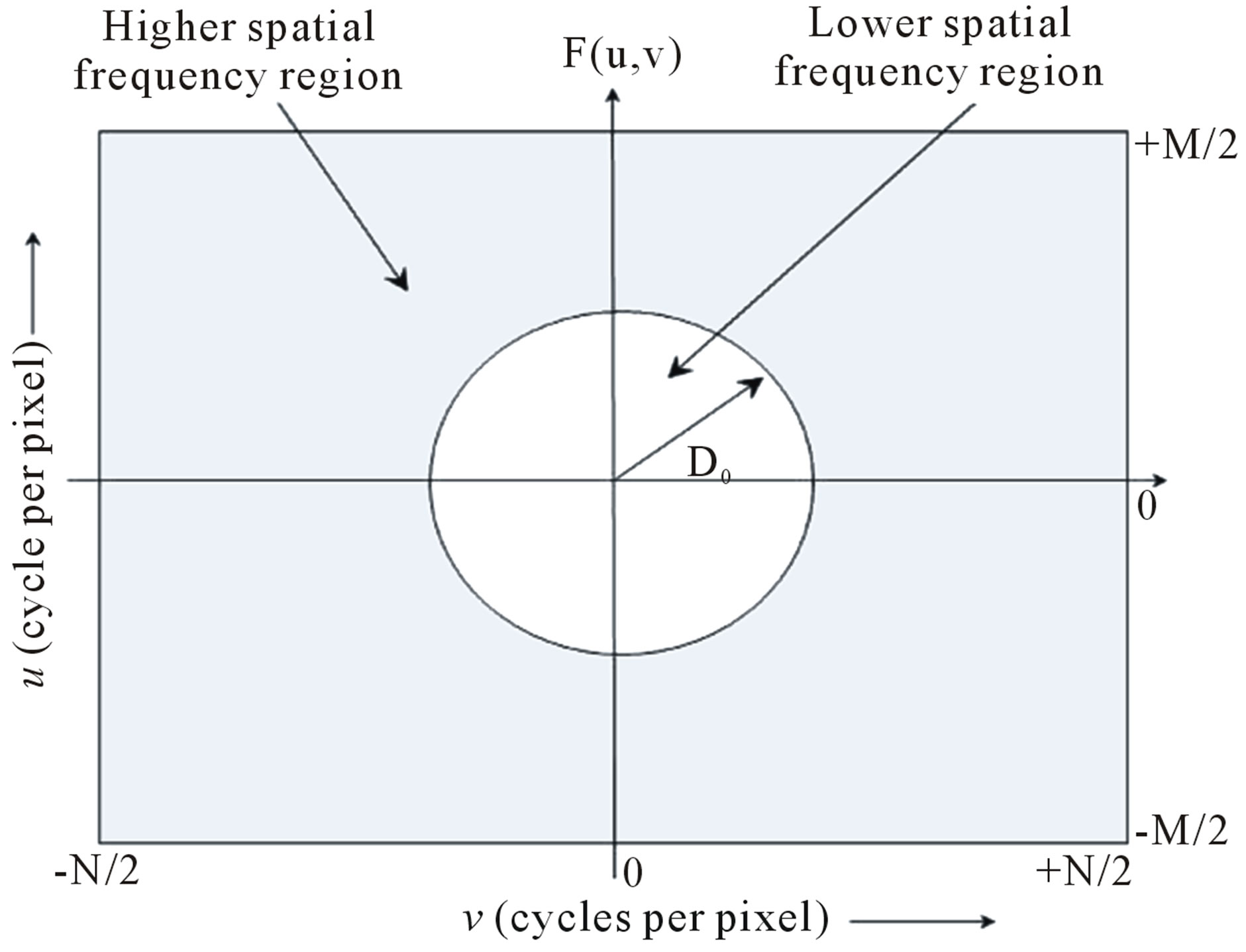
Figure 3. Fourier spectrum, F(u, v), of an image showing higher and lower spatial frequency regions.
for comparison. The procedure is repeated for all the subjects with ICH considered under study, and finally the image signal intensity RHFP values are evaluated.
Statistical analysis was carried out using excel program and SPSS 17.0 software package. The results were tested for statistical significant difference between the HFP values obtained for the subjects with ICH and their contralateral normal hemisphere. Similarly the statistical significant difference between the RHFP values obtained for the subjects with ICH across the four different stages was tested. The analysis was carried out at 99% confidence level (p < 0.01) with z test, using the significant difference of means method [29]. The correlation between the RHFP values and the different stages of ICH was evaluated.
3. RESULTS AND DISCUSSIONS
DW image of a subject showing ICH in area 3 and at axial section 14 is shown in Figure 4. The plot of the spatial variation of intensity distribution for a sub-region of the ROI (area 3, axial section 14) resulting in maximum HFP value, for the subject indicated in Figure 4, is shown in Figure 5. The corresponding power spectrum is shown in Figure 6. It is observed from Figure 5 that the spatial intensity variation distribution for the subject with ICH has abrupt jumps, and this leads to higher value of the higher spatial frequency component out of the total power spectrum. Similarly Figures 7 and 8, respectively, show the plots of the spatial variation of intensity distribution and the power spectrum for the corresponding sub-region on the contralateral normal hemisphere for the same subject. The spatial intensity variation distribution is almost uniform in the contralateral normal hemisphere as shown in Figure 7, and this leads to a considerable smaller value of the higher spatial frequency
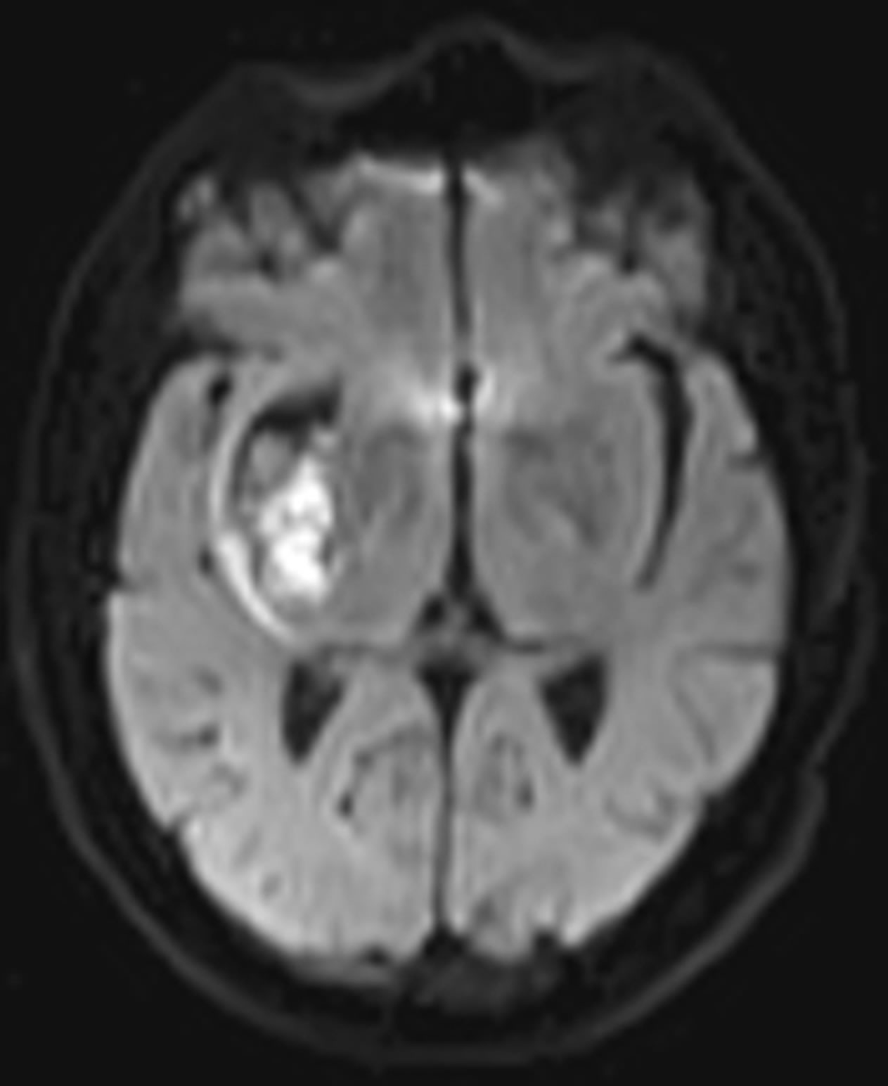
Figure 4. Axial DW image showing ICH (area 3, axial section 14).
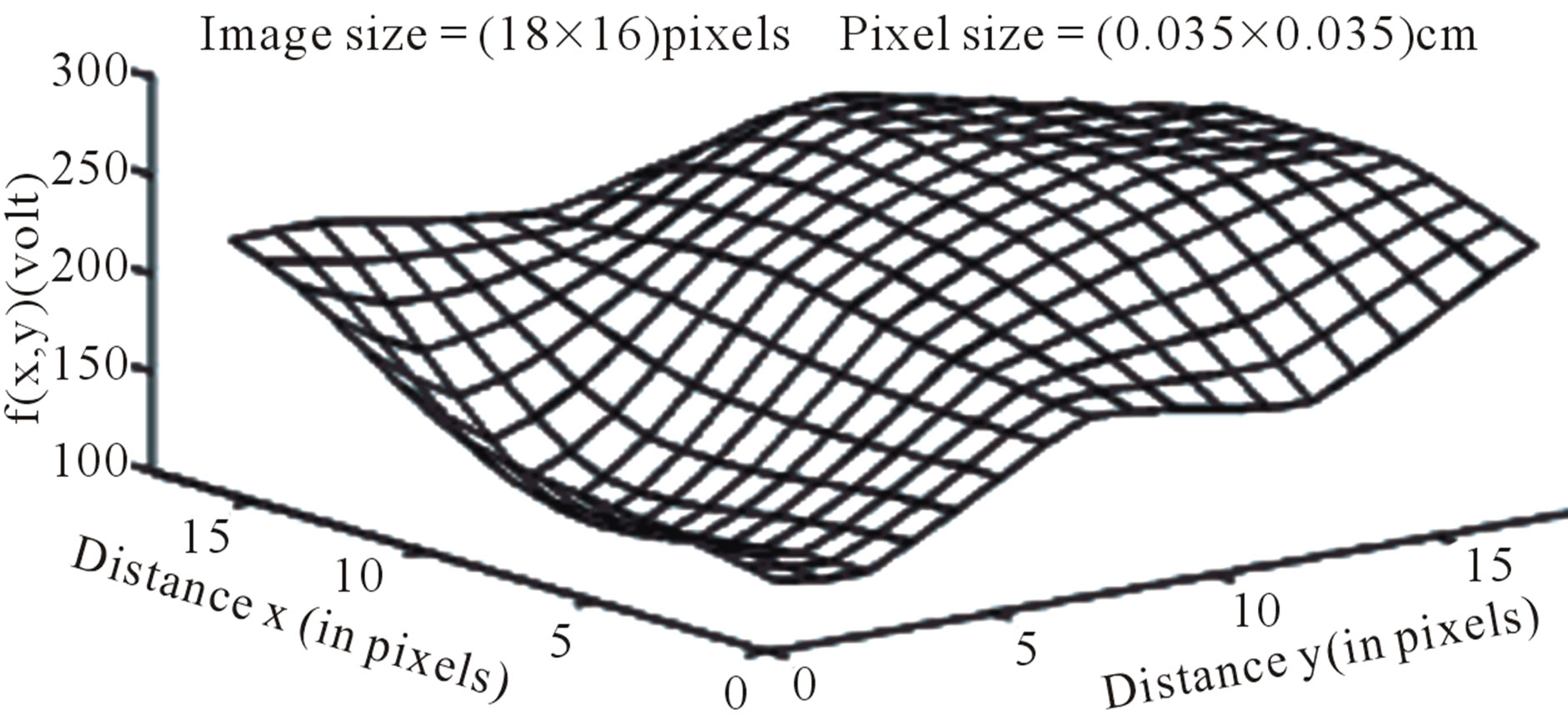
Figure 5. Image intensity distribution for the subject with ICH (area 3, axial section 14).
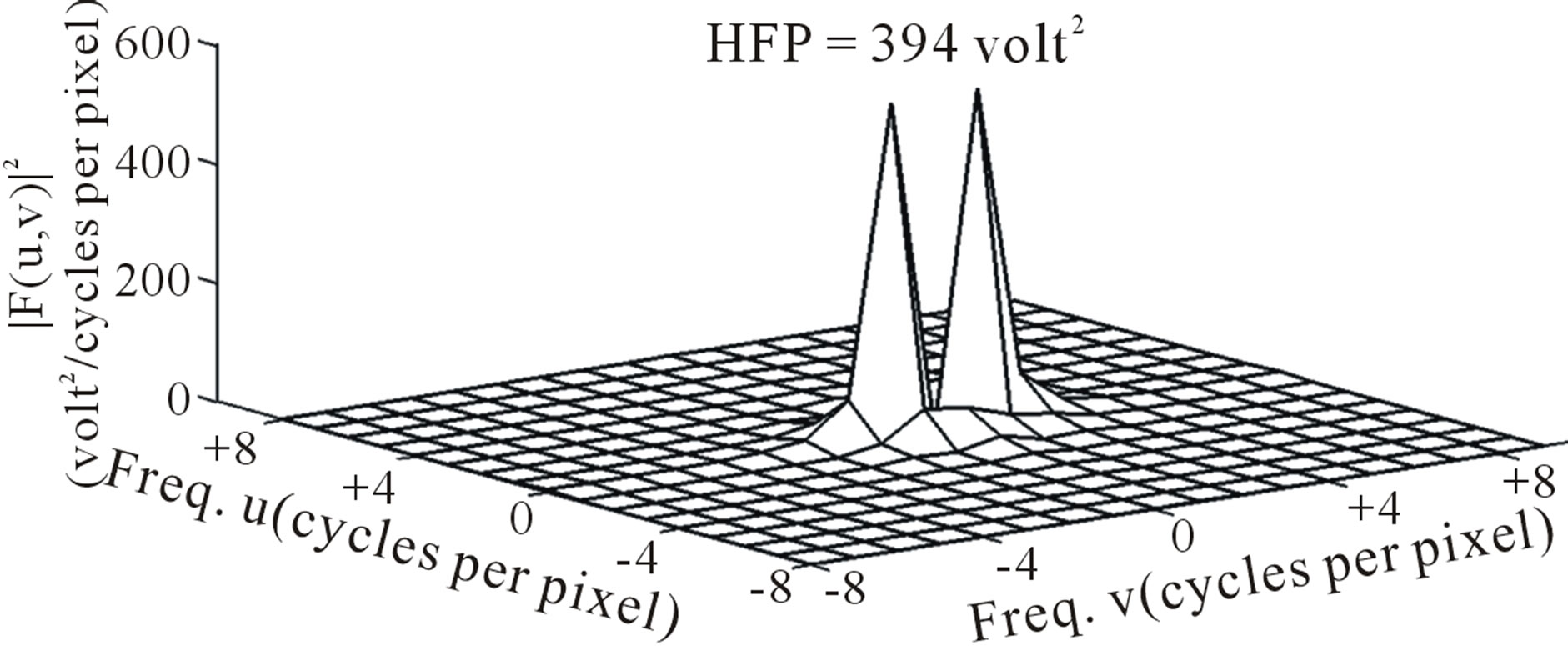
Figure 6. Power spectrum (after deleting the DC component) for the subject with ICH (area 3, axial section 14).
component out of the total power spectrum as shown in Figure 8. Consequently maximum HFP value for the subject with ICH (394 volt2) is much elevated as shown in Figure 6 compared to that of the contralateral normal hemisphere (0.671 volt2) as shown in Figure 8. The maximum HFP value evaluated from the subject with ICH indicates the maximum change in the image intensity variation across the selected ROI at axial section 14, and also indicates its exact location, (5, 16), in the (x, y) co-ordinates (Figure 5).
The semilog plot of the variation in the maximum image signal intensity HFP values (decisive HFP values) and the corresponding image signal intensity HFP values on the contralateral normal hemisphere, for all the 30 subjects considered in the present study is shown in Figure 9. The difference in the maximum image signal intensity HFP values for the subjects with ICH compared to their contralateral normal hemispheres, were highly significant (p < 0.01) in the areas of the brain, where there was a high incidence of haemorrhage. Results suggest that the maximum image signal intensity HFP values obtained from DW images, for the subjects with ICH can be used to clearly differentiate the ICH subjects from the normal subjects.
Table 1 lists the range of the maximum image signal intensity HFP values obtained from the subjects with ICH and their corresponding HFP values on the contralateral normal hemisphere, across different stages of ICH. Also the range of the RHFP values evaluated across the different stages of ICH is listed. The variation in the mean RHFP value within each stage of ICH (last column
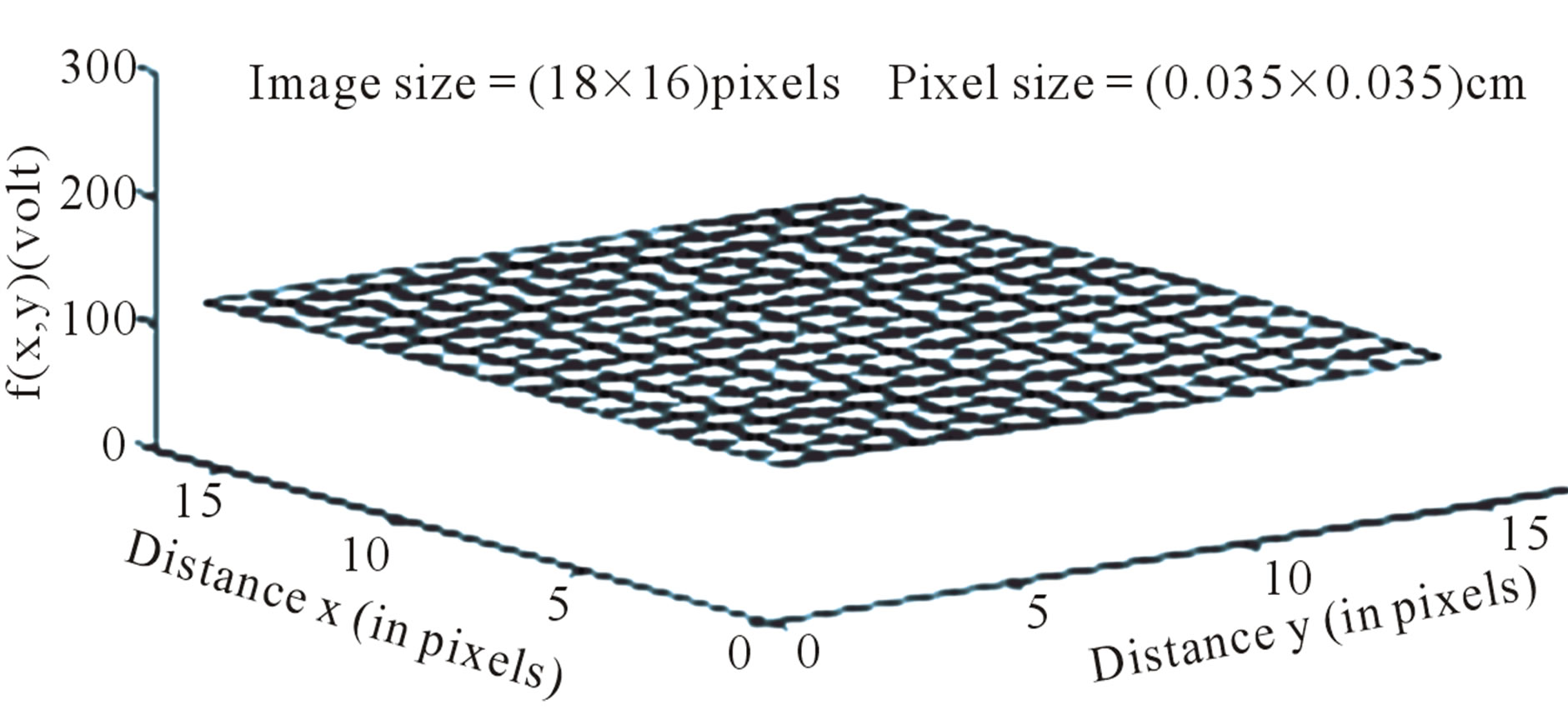
Figure 7. Image intensity distribution on the contralateral hemisphere.
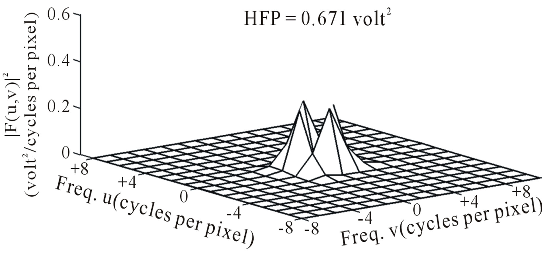
Figure 8. Power spectrum (after deleting the DC component) on the contralateral hemisphere.
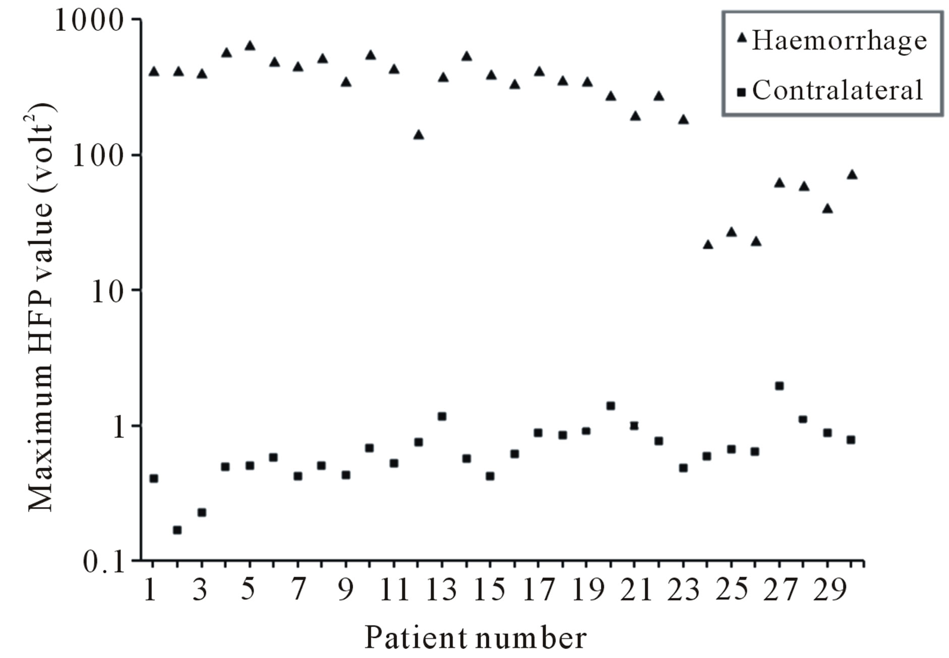
Figure 9. Variation in the maximum HFP (semilog plot) for ICH subjects and the corresponding HFP on the contralateral normal hemisphere.
of Table 1) is as plotted in Figure 10.
It is observed that the RHFP values are notably high for Stage 1: Hyperacute (<1 day) of ICH. Further there is a subsequent decrease in the RHFP values from Stage 2: Acute (1 - 7 days) to Stage 3: Late subacute (7 - 14 days) of ICH and they reach their minimum for Stage 4— Chronic (>14 days). Therefore, we quantitatively confirm that ICH is mainly hyper-intense on DW images in the Stage 1: Hyperacute (<1 day) resulting in high values of RHFP. Evolution into the Stage 2: Acute (1 - 7 days) and Stage 3: Late subacute (7 - 14 days) is identified by reduction in signal intensity and corresponding lowering of the RHFP values. The Stage 4: Chronic (>14
Table 1. Maximum HFP and Mean RHFP* values in different stages of ICH.
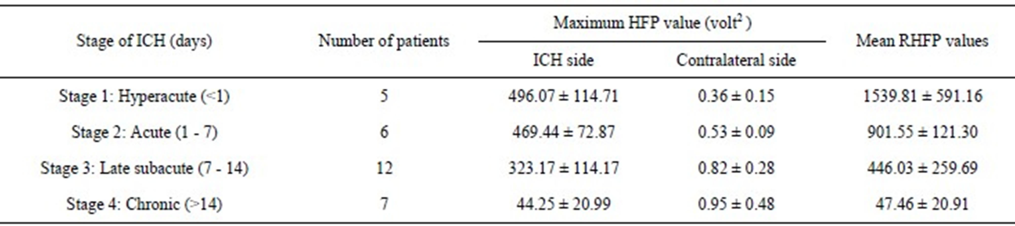
*RHFP = (maximum HFP on ICH side − corresponding HFP on contralateral side)/(corresponding HFP on contralateral side)
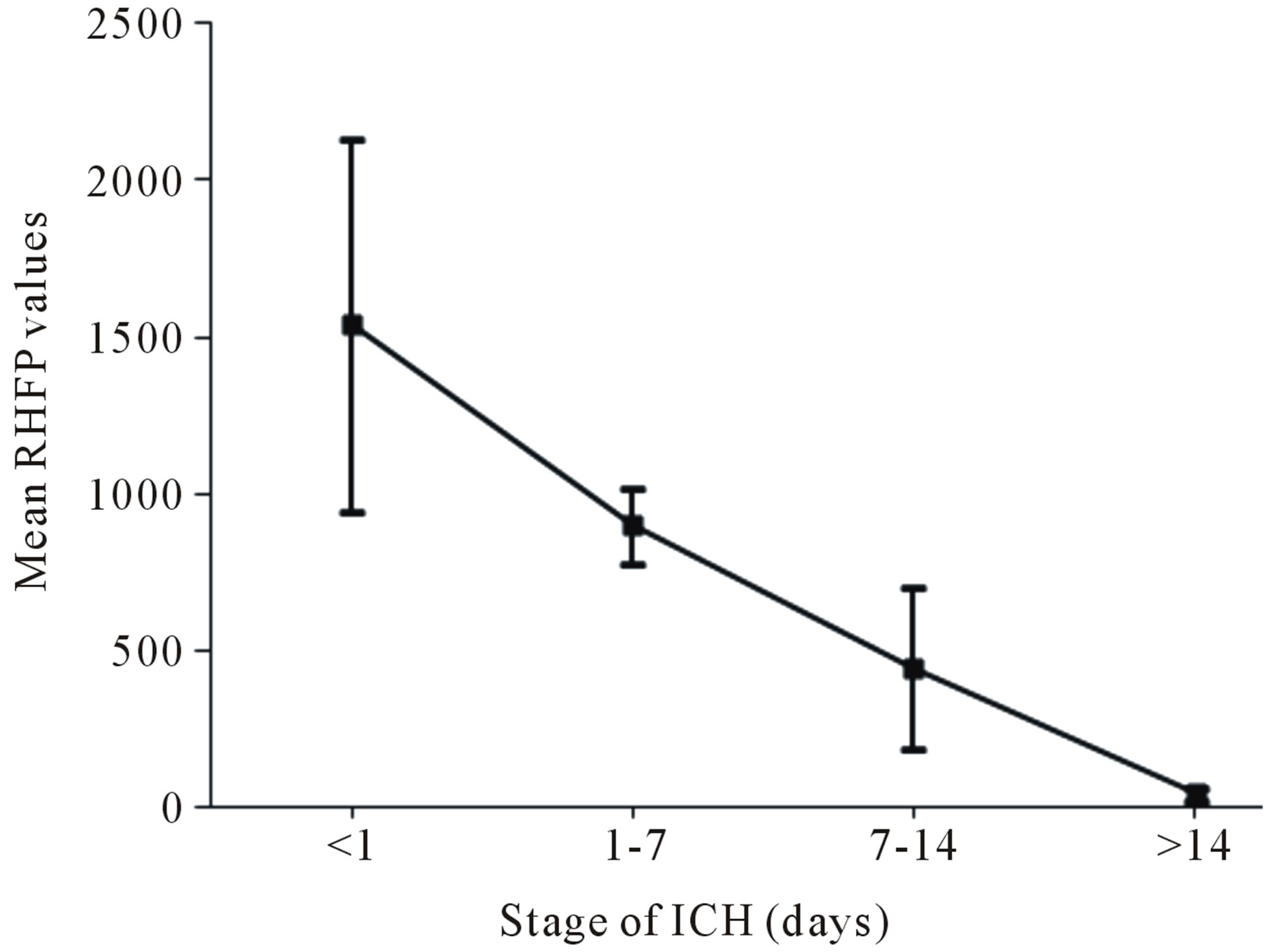
Figure 10. Variation in the mean RHFP values with the stage of ICH.
days) shows marked hypo-intensity and thereby results in the lowest values of RHFP. There was a significant difference observed between the RHFP values across different stages of ICH (p < 0.05 between Stage 1 and Stage 2 and p < 0.01 between all the other stages of ICH).
The plot of the variation in the RHFP values with the stage of ICH for all the 30 subjects considered in our study is shown in Figure 11. The line given by the equation y = −2.55*x + 1254.02, represents the linear regression that fit the data. A negative correlation of the order of r = −0.81 was found between the RHFP values and the different stages of ICH, which is an indicator that early stages of ICH gives rise to higher values of RHFP. The progress in the RHFP values for the different stages of ICH is indicative that it can be helpful in the characterization of ICH and can positively be instructive in differentiating the various stages of ICH.
The results obtained in our study agree with the findings of the previously published work on the signal intensity variations of the haemorrhage on DW images [6,9,18,19]. Investigators in the past have also reported the evolution of haemorrhage using the ADC values [15,16]. However in contrast to the work carried out in the past, wherein only a particular affected axial section
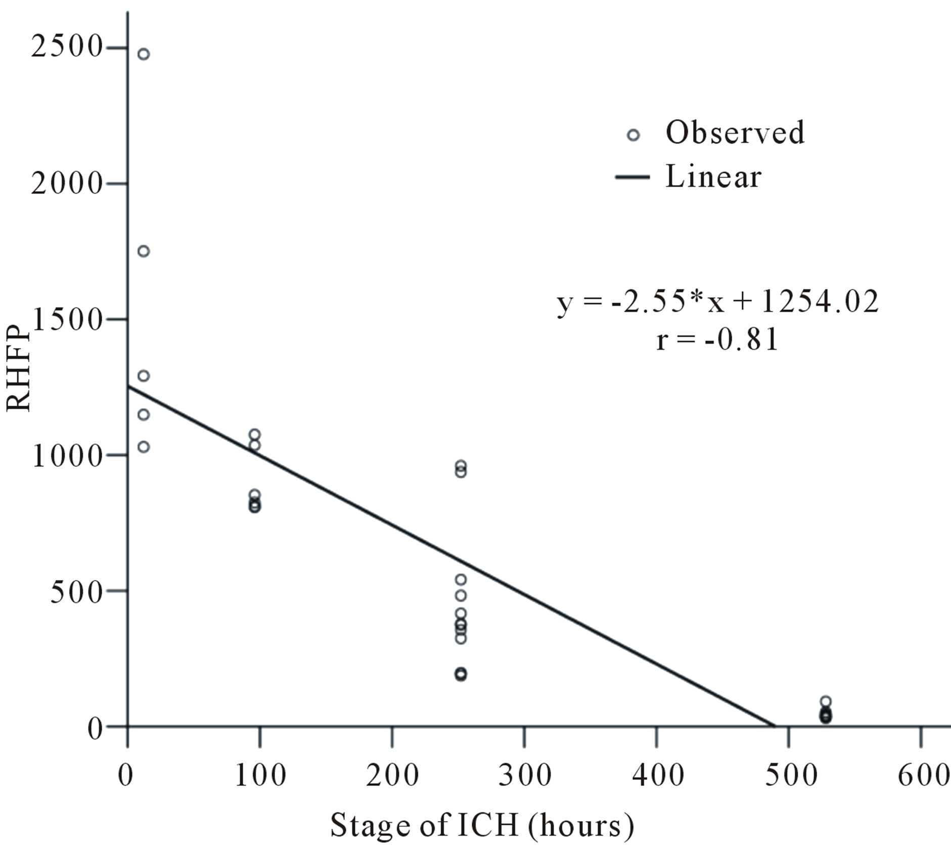
Figure 11. Variation in the RHFP values with the stage of ICH.
on DW image is considered for analysis, we include all the affected axial sections to arrive at the decisive value for RHFP. Additionally we include the entire affected area on each axial section selected for the analysis in contrast to the ADC methods, wherein, evaluations are done by considering a small region within the affected area.
4. CONCLUSION
Analysis of the results indicate that the image signal intensity changes on DW images for the subjects with ICH can be employed to markedly distinguish them quantitatively from the normal subjects. The relative increase in the image signal intensity HFP values on DW images for the subjects with ICH compared to their contralateral normal hemisphere were in the range of (31.0 - 2477.32). The quantitative changes in the values of the image signal intensity HFP parameter can be assessed and probably used to identify the different stages of ICH, so that early changes taking place in the brain can be detected. This can positively assist neurosurgeons in determining the severity of the brain haemorrhage, to consider early remedial methods and in predicting recovery.
5. ACKNOWLEDGEMENTS
The authors would like to thank Dr. Sudhir Pai (Sr. Consultant, Neurosurgeon, Vikram Hospital, Bangalore, India) for his valuable assistance in data collection and Dr. Deepak Y. S. (D.N.B. Resident, RAGAVS Diagnostic and Research Center, Bangalore, India) for his helpful and constructive suggestions during the planning and development of this research work.
REFERENCES
- Andersen, K.K., Olsen, T.S., Dehlendorff, C. and Kammersgaard, L.P. (2009) Hemorrhagic and ischemic strokes: Compared stroke severity, mortality, and risk factors. Stroke, 40, 2068-2072. doi:10.1161/STROKEAHA.108.540112
- Qureshi, I., Tuhrim, S., Broderick, J.P., Batjer, H.H., Hondo, H. and Hanley, D.F. (2001) Spontaneous intracerebral haemorrhage. The New England Journal of Medicine, 344, 1450-1460. doi:10.1056/NEJM200105103441907
- Kidwell, S., Chalela, J.A., Saver, J.L., Starkman, S., Hill, M.D., Demchuk, A.M., Butman, J.A., et al. (2004) Comparison of MRI and CT for detection of acute intracerebral haemorrhage. Journal of American Medical Association, 292, 1823-1830. doi:10.1001/jama.292.15.1823
- Chalela, J.A., Kidwell, C.S., Nentwich, L.M., Luby, M., Butman, A., Demchuk, A.M., Hill, M.D., et al. (2007) Magnetic resonance imaging and computed tomography in emergency assessment of patients with suspected acute stroke: A prospective comparison. The Lancet, 369, 293- 298. doi:10.1016/S0140-6736(07)60151-2
- Schellinger, P.D., Jansen, O., Fiebach, J.B., Hacke, W. and Sartor, K. (1999) A standardized MRI stroke protocol: Comparison with CT in hyperacute intracerebral haemorrhage. Stroke, 30, 765-768. doi:10.1161/01.STR.30.4.765
- Smith, E.E., Rosand, J. and Greenberg, S.M. (2006) Imaging of hemorrhagic stroke. Magnetic Resonance Imaging Clinics, 14, 127-140. doi:10.1016/j.mric.2006.06.002
- Gomori, J.M., Grossman, R.I., Goldberg, H.I., Zimmerman, R.A. and Bilaniuk, L.T. (1985) Intracranial hematomas: Imaging by high-field MR. Radiology, 157, 87-93.
- Atlas, S.W. and Thulborn, K.R. (1998) MR detection of hyperacute parenchymal haemorrhage of the brain. American Journal of Neuroradiology, 19, 1471-1477.
- Bradley, W.J. (1993) MR appearance of haemorrhage in the brain. Radiology, 189, 15-26.
- Atlas, S., Mark, A., Grossman, R. and Gomori, J. (1998) Intracranial haemorrhage: Gradient-echo MR imaging at 1.5 T comparison with spin-echo imaging and clinical applications. Radiology, 168, 803-807.
- Patel, M.R., Edelman, R.R. and Warach, S. (1996) Detection of hyperacute primary intraparenchymal haemorrhage by magnetic resonance imaging. Stroke, 27, 2321- 2324. doi:10.1161/01.STR.27.12.2321
- Chabert, S. and Scifo, P. (2007) Diffusion signal in magnetic resonance imaging: Origin and interpretation in neuro-sciences. Biological Research, 40, 385-400. doi:10.4067/S0716-97602007000500003
- Le Bihan, D. (2003) Looking into the functional architecture of the brain with diffusion MRI. Nature Reviews Neuroscience, 4, 469-480. doi:10.1038/nrn1119
- Rajeshkannan, R., Moorthy, S., Sreekumar, K.P., Rupa, R. and Prabhu, N.K. (2006) Clinical applications of diffusion weighted MR imaging: A review. Indian Journal of Radiology and Imaging, 16, 705-710. doi:10.4103/0971-3026.32328
- Atlas, S.W., DuBois, P., Singer, M.B. and Lu, D. (2000) Diffusion measurements in intracranial hematomas: Implications for MR imaging of acute stroke. American Journal of Neuroradiology, 21, 1190-1194.
- Hideichi, T., Masahito, K., Sadao, S., Fumiko, S. and Ban, M. (1999) Cerebral haemorrhage. Serial study using diffusion-weighted MRI. Japanese Journal of Stroke, 21, 245-252. doi:10.3995/jstroke.21.245
- Ebisu, T., Tanaka, C., Umeda, M., Kitamura, M., Fukunaga, M., Aoki, I., Sato, H., et al. (1997) Hemorrhagic and nonhemorrhagic stroke: Diagnosis with diffusion weighted and T2-weighted echo-planar MR imaging. Radiology, 203, 823-828.
- Silvera, S., Oppenheim, C., Touzé, E., Ducreux, D., Page, P., Domigo, V. and Mas, J.L. (2005) Spontaneous intracerebral hematoma on diffusion-weighted images: Influence of T2-shine through and T2-blackout effects. American Journal of Neuroradiology, 26, 236-24.
- Kang, K., Na, D.G., Ryoo, J.W., Byun, H.S., Roh, H.G. and Pyeun, Y.S. (2001) Diffusion-weighted MR imaging of intracerebral haemorrhage. Korean Journal of Radiology, 2, 183-191. doi:10.3348/kjr.2001.2.4.183
- Stadnik, T.W., Demaerel, P., Luypaert, R.R., Chaskis, C., Van Rompaey, K.L., Michotte, A. and Osteaux, M.J. (2003) Imaging tutorial: Differential diagnosis of bright lesions on diffusion-weighted MR images. Radiographic, 23, 686.
- Attia, S., El Khatib, M.G., Bilal, M. and Nassar, H. (2007) Spontaneous intracerebral hematoma in young people: Clinical and radiological magnetic resonance imaging features by diffusion-weighted images. Egyptian Journal of Neurology, Psychiatry and Neurosurgery, 44, 561- 576.
- Maldjian, J.A., Listerud, J., Moonis, G. and Siddiqi, F. (2001) Computing diffusion rates in t2-dark hematomas and areas of low t2 signal. American Journal of Neuroradiology, 22, 112-118.
- Linfante, I., Llinas, R.H., Caplan, L.R. and Warach, S. (1999) MRI features of intracerebral hemorrhage within 2 hours from symptom onset. Stroke, 30, 2263-2267. doi:10.1161/01.STR.30.11.2263
- Felber, S., Auer, A., Wolf, C., Schocke, M., Golaszewski, S., Amort, B. and ZurNedden, D. (1999) MRI characteristics of spontaneous intracerebral hemorrhage. Radiologe, 39, 838-846. doi:10.1007/s001170050720
- Gonzalez, R.C. and Wintz, P. (1987) Image transforms in “Digital Image Processing,” 2nd Edition, Addison-Wesley, New York.
- Kulkarni, D.A., Bhagyashree, S.M. and Udupi, G.R. (2010) Texture analysis of mammographic images. International Journal of Computer Applications, 5, 12-17.
- Prabhu, K.G., Patil, K.M. and Srinivasan, S. (2001) Diabetic Feet at Risk: A new method of analysis of walking foot pressure images at different levels of neuropathy for early detection of plantar ulcers. Medical and Biological Engineering and Computing, 39, 288-293. doi:10.1007/BF02345282
- Charanya, G., Patil, K.M., Thomas, V.J., Narayanamurthy, V.B., Parivalavan R. and Visvanath, K. (2004) Standing foot pressure image analysis for variations in foot sole soft tissue properties and levels of diabetic neuropathy. ITBM-RBM, 25, 23-33. doi:10.1016/j.rbmret.2003.11.002
- Gupta, S.C. and Kapoor, V.K. (1982) Fundamentals of mathematical statistics. 11th Edition, Sultan Chand and Sons, New Delhi.
NOTES
*Retired.