iBusiness
Vol.2 No.2(2010), Article ID:1957,12 pages DOI:10.4236/ib.2010.22019
Comparison of GA Based Heuristic and GRASP Based Heuristic for Total Covering Problem
![]()
1Network Coordination, BSNL, Chennai, India; 2Department of Management Studies, School of Management, Pondicherry University, Pondicherry, India.
Email: vijeyamurthy@gmail.com, Panneer_dms@yahoo.co.in
Received January 25th, 2010; revised March 3rd, 2010; accepted April 9th, 2010.
Keywords: Genetic Algorithm, GRASP, Total covering problem, Boolean Operators, Care and share operator
ABSTRACT
This paper discusses the comparison of two different heuristics for total covering problem. The total covering problem is a facility location problem in which the objective is to identify the minimum number of sites among the potential sites to locate facilities to cover all the customers. This problem is a combinatorial problem. Hence, heuristic development to provide solution for such problem is inevitable. In this paper, two different heuristics, viz., GA based heuristic and GRASP based heuristic are compared and the best is suggested for implementation.
1. Introduction
Consider a sales region of a product, which in turn has different customer regions. The company selling the product should fix necessary number of dealer points such that the customers in that sales region are fully served. The company may fix a maximum of say 5 km of distance for the customers to reach a given dealer point from his/her region (customer region). In this process, a given customer may be covered by more than one dealer point. The objective is to locate the minimum number of dealer points in the sales region under consideration such that those dealer points cover all the customers regions.
Here, the process of serving a customer region by a dealer point is called as covering that customer region by that dealer point. The word “cover” means that the location of a customer is well within the given upper limit for the distance from a facility-location from where that customer will be served. Here, the objective is to locate facilities at minimum number of sites to cover all the customers. Such problem is known as total covering problem [1].
Consider a problem in which dealer points are to be located to serve the customers in a sales region. Assume that there are six customer regions, which are to be covered by dealer points. In this problem, five potential locations are identified for locating dealer points. The distance matrix between the customer regions is as shown in Table 1.
Now, a distance criterion of say, 5 km is assumed. This means that no region in the sales region is beyond 5 km from a site where a dealer is located. Based on this assumption, a covering coefficient is defined as shown below.
Let,  , if
, if 
 , otherwise where, cij is the covering coefficient for the customer region i and the potential dealer point j and dij is the distance between the customer region i and the potential dealer point j. Based on this definition of covering coefficient, the corresponding covering coefficient matrix is shown in Table 2.
A careful examination of the Table 2 reveals that if the potential site 1 and the potential site 3 are assigned with dealers, all the six customer regions in the sales regions will be fully covered. As per this coverage, the potential site 1 will cover the customer regions 1, 2 and 4 and the potential site 3 will cover the customer regions
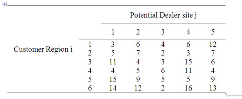
Table 1. Distance matrix of locating dealer points (distance in km)
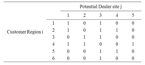
Table 2. Covering coefficients matrix of locating dealer points
1, 2, 3, 5 and 6. The customer regions 1 and 2 are covered by the facilities from both the selected potential sites. This is an example of multiple-coverage of some custommers by a set of facilities. The different examples of total covering problem are shown in Table 3. The total covering problem falls under combinatorial category. Hence, it is inevitable to design an efficient heuristic to obtain near optimal solution. In this paper, an attempt has been made to develop and compare a genetic algorithm based heuristic and a GRASP based heuristic for the total covering problem.
2. Review of Literature
The covering problem comes under the facilities location problem. The covering problem can be classified into total covering problem and partial covering problem. The objective of the total covering problem is to cover all the customers with the minimum number of facilities whereas the objective of the partial covering problem is to cover as many customers as possible with the minimum number of facilities without exceeding the limit on the utmost number of facilities to be operated as suggested by the management. In this research, the total covering problem is considered.
Toregas et al. [2] have developed a liner programming model to solve the traditional set covering problem with equal cost in the objective function. Patel [3] has used dynamic programming approach for locating rural social service centers for the Dharampur taluka in South Gujarat in India. Klastorin [4] has solved the conventional set-covering problem by mapping it into an assignment problem. Saatcioglu [5] has used a mathematical model for airport site selection based on Turkish data. Neebe [6]
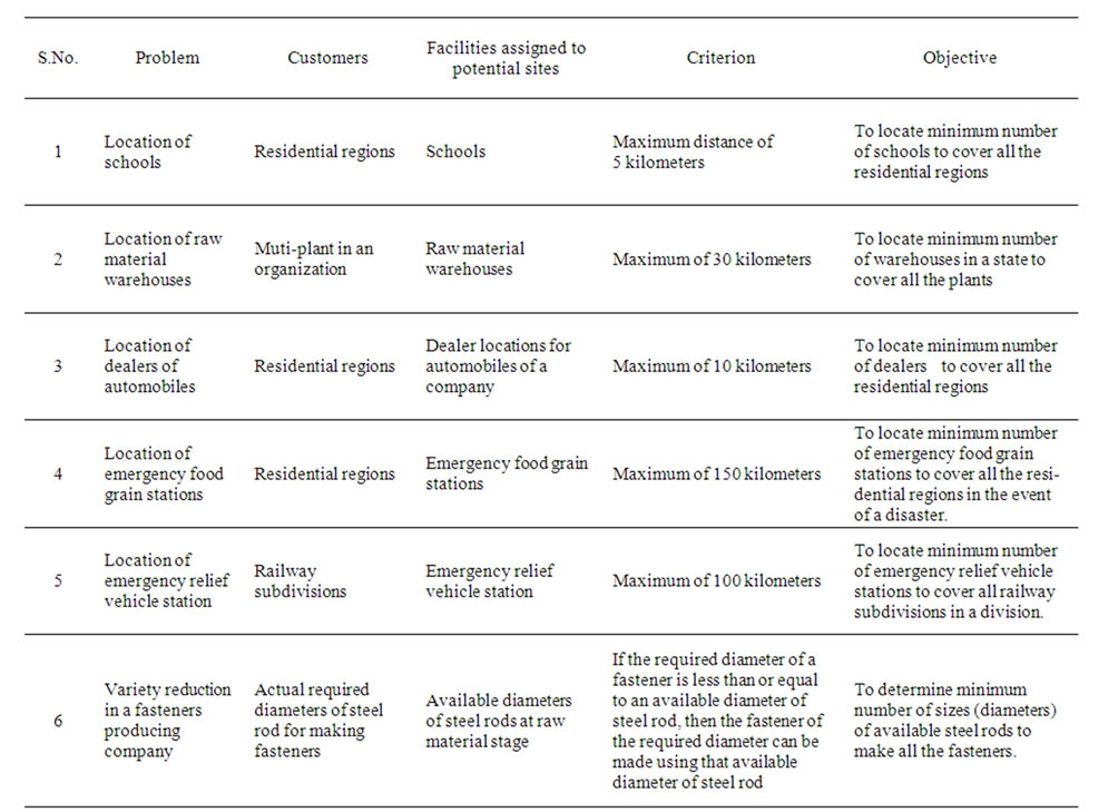
Table 3. Examples of total covering problem
has developed a procedure for locating emergency-service facilities for all possible response distances. Panneerselvam [7] has developed a heuristic procedure for the total covering problem. Rajkumar and Panneerselvam [8] have improved the work of Panneerselvam [7]. Later, Panneerselvam [9] has developed an efficient heuristic for the total covering problem. O’kelly [10] demonstrated the use of covering problem for locating interacting hub facilities. Hubs are central facilities, which act as switching points in networks connecting a set of interacting nodes. Boffey [11] has discussed the location problems arising in computer networks.
Chan et al. [12] have developed a branch and bound algorithm with multiplier adjustment for the traditional set-covering problem. Chaovalitwongse, Berger-Wolf, Dasgupta and Ashley [13] have conducted a simulation study of their proposed algorithm to demonstrate that their combinatorial approach is reasonably accurate. The results suggests the proposed algorithm would pave a way to a new approach in computational populations genetics as it does not require any a priori knowledge about allele frequency, population size, mating system or family size distributions to reconstruct sibling relationships. To extract the minimum number of biologically consistent sibling groups, the proposed combinatorial approach is employed to formulate this minimization problem as a set covering problem.
Pelegrin, Redondo, Fernandez, Garcia and Ortigosa [14] have proposed genetic like algorithm, GASUB for finding the global optima to discrete location problems. The authors claim that the algorithm finds the predetermined number of global optima, if they exist, for a variety of discrete location problems. GASUB has been compared to MSH, the multi start substitution method and found that it gave better solutions than MSH. Alumur, Kara and Karasan [15] have classified and surveyed the hub location models, including the recent trends on hub location and provided a synthesis of the literature. The hub location problem is concerned with locating hub facilities and allocating demand nodes to hubs in order to route the traffic between origin-destination pairs. Hubs are special facilities that serve as switching, transshipment and sorting points in many—to—many distribution systems.
Marianov, Mizumori and Re Velle [16] proposed a new heuristic, called heuristic concentration—integer (HCI). The authors have applied the algorithm to the maximal availability location problem (MALP) and the solutions are compared to those obtained using linear programming with branch and bound. They claim that HCI could find good solutions to the problems in a reasonable time compared to LP-IP solutions. Francisco, Antonio and Glaydston [17] have presented a solution procedure for probabilistic model using column generation having constraint in waiting time, queue length for congested system with one or more servers per service center for the maximal covering location—allocation problems. The authors claim that the results were obtained in reasonable time. Batanovic, D. Petrovic and R. Petrovic [18] have considered the maximum covering location problems in networks in uncertain environments. They have proposed three new algorithms for choosing the best facility locations assuming that the demands at all nodes are equally important, the relative weights of demands at nodes are deterministic and weights of demand at nodes are imprecise. The algorithms are based on searching among potential facility nodes by applying comparison operations on discrete fuzzy sets.
The review of literature indicates that the researchers have developed mathematical models, branch and bound algorithms and heuristics. Since, the total covering problem comes under combinatorial category, the development of an efficient heuristic is inevitable. In this paper, the researchers have proposed a genetic algorithm based heuristic and a GRASP based heuristic for total covering problem and compared their performances.
3. Mathematical Model of Total Covering Problem
In general, all emergency/ essential service related situations are formulated as total covering problems.
A mathematical model of the total covering problem is presented below.
Let, m be the number of customers;
n be the number of potential sites;
cij be the covering coefficient for the customer i and potential site j Minimize 
Subject to
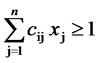 for i = 1 to m.
wherexj = 1, if the potential site j is assigned with a facility;
= 0, otherwise, for j = 1, 2, 3,…, n.
The objective function minimizes the total number of sites selected for assigning facilities. The constraint i ensures that each customer is served/covered by at least one selected potential site which is assigned with a facility.
4. Development of Heuristics
The total covering problem falls under combinatorial category. Hence, it is inevitable to design an efficient heuristic to get near optimal solution. In this paper, the authors have made an attempt to develop a Genetic Algorithm (GA) based heuristic and a Greedy Randomized Adaptive Search Procedure (GRASP) based heuristic to obtain global optimum solution for the total covering problem.
4.1 GA Based Heuristic
Genetic algorithm is a meta-heuristic, which is used to find the solution to any combinatorial problem. It mimics the mechanism of selection and evolution. In order to achieve the objective, GA generates successive population of alternate solutions until obtaining a solution, which yields acceptable result. Within the generation of each successive operation, an improvement in the quality of the individual solution is achieved. Hence, GA can quickly move to a successful outcome without determining every possible solution to the problem. The procedure used in the genetic algorithm is based on the fundamental processes that control the evolution of biological organisms, namely, natural selection and reproduction.
Organism’s ability to survive within its environment is improved by the two processes as explained below.
1) Natural selection determines which organism has the opportunity of reproduction and survival within a population.
2) Reproduction involves genes from two separate individuals combining to form offspring that inherit the survival characteristics of their parents.
This section presents a genetic algorithm based heuristic for total covering problem. The genetic algorithm has two major operations, viz. crossover operation and mutation. Consider the covering coefficient matrix, which is already shown in Table 2 and the same is reproduced in Table 4.
4.1.1 Crossover Operation
In this section, the crossover operation which is performed on two chromosomes to produce offspring is presented. To explain this operation, the encoding of the given covering coefficient data into chromosomes is as presented below.
The 0-1 entries in each of the rows of the covering coefficient matrix are treated as a chromosome. A zero entry in a chromosome represents non-allocation of facility to the respective potential site and one entry in that chromosome represents allocation of facility to the respective potential site. So, the sequence of 0-1 entries in each chromo
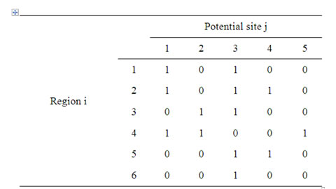
Table 4. Covering Coefficients Matrix of Locating Dealers
some represents the values of the decision variable xj, for j = 1, 2, 3, …, n, where xj = 1 if the potential site j is assigned with a facility; otherwise, it is equal to 0 and n is the total number of potential sites. So, entries in each chromosome give one possible solution to the total covering problem.
If the given problem has m customers, then the initial population will have m chromosomes. For the given problem, the chromosomes of the initial population are as listed below and each chromosome is treated as a binary number.
Chromosome 1: 1 0 1 0 0 Chromosome 2: 1 0 1 1 0 Chromosome 3: 0 1 1 0 0 Chromosome 4: 1 1 0 0 1 Chromosome 5: 0 0 1 1 0 Chromosome 6: 0 0 1 0 0 The crossover operation is done using the following pairs of Boolean operators:
1) Logic OR and Logic AND 2) Odd shift before Logic OR and Logic AND 3) Even shift before Logic OR and Logic AND 4) Logic OR and odd shift before Logic OR 5) Logic OR and even shift before Logic OR 6) Logic AND and odd shift before Logic AND 7) Logic AND and even shift before Logic AND While the offspring are created using the above pairs of crossover operators, if any one offspring is infeasible, then it is replaced with a feasible offspring, which will be created by Care and Share crossover operation.
4.1.2 Evaluation of Offspring
Consider an offspring “1 0 1 0 0”. Its evaluation is done as presented in Figure 1" target="_self"> Figure 1. The genes of the offspring are positioned in the respective order just above the columns corresponding to potential sites. The regions which are covered by each site, which is assigned with a facility are shown by marking squares around the respective “1” entries in the covering coefficient matrix. In Figure 1, the site 1, which is assigned with a facility, covers the regions 1, 2 and 4. The facility assigned at the site 3 covers the regions 1, 2, 3, 5 and 6. The union of the subsets of regions, which are covered by the site 1 and the site 3 are {1, 2, 3, 4, 5, 6}. This means that all the six regions are covered by the facilities that are assigned at the site 1 and the site 3. Hence, the offspring is a feasible offspring. The corresponding fitness function value (number of sites which are assigned with facilities) is 2.
4.1.3 Care and Share Crossover Operation
Consider another offspring, whose genes are “0 1 0 0 0”. As explained in section 4.1.2, the coverage of the regions by the only site 2 in this offspring, which is assigned with a facility, is shown in Figure 2. In Figure 2, the facility which is assigned at the site 2 covers only the regions 3 and 4. So, the solution of this offspring is infeasible. Now, the set of selected sites for assigning facility = {2}. Then, another sub-covering coefficient matrix with the remaining potential sites (1, 3, 4 and 5) and remaining regions (1, 2, 5 and 6) is shown in Figure 3. Now find the maximum number of regions that can be covered by any unselected potential site from Figure 3. The corresponding value in Figure 3 is 4, which occurs for the potential site 3. So, include it in the set of selected sites for assigning facilities as shown: Set of selected sites for assigning facilities = {2, 3}.
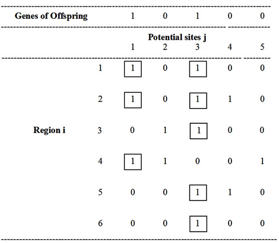
Figure 1. Coverage of regions by Offspring “1 0 1 0 0 ”
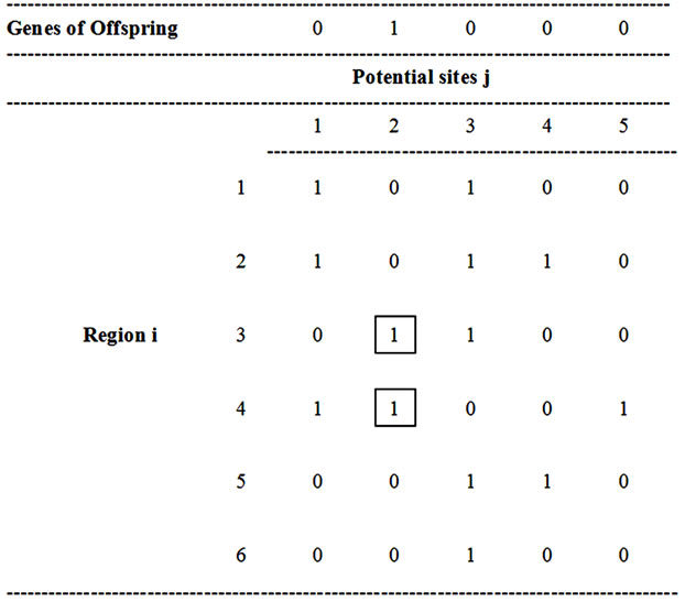
Figure 2. Coverage of regions by Offspring “ 0 1 0 0 0”
From Figure 3, it is visible that the facility, which is assigned at the potential site 3 can cover all the regions (1, 2, 4 and 5) in it. So, there is no more uncovered region. The modified offspring for the given offspring is constructed by having 1 in the position 2 and position 3 and 0 in the remaining positions as shown below.
Modified offspring = {0 1 1 0 0}
Now, the earlier offspring, {0 1 0 0 0} is to be substituted with the modified offspring, {0 1 1 0 0}. The process of constructing a feasible offspring for an infeasible offspring is called “Care and Share” crossover operation. In this example, Figure 3 itself gives the feasible offspring. In general, the process of forming sub-covering coefficient matrices is to be continued until all the regions are covered.
4.1.5 Mutation
Mutation is a process of randomizing the genes in each chromosome. In a chromosome, this can be done by randomly selecting any two genes in it and swapping them. Since, the usage of Logic AND makes many zeros in offspring, some of the offspring will become infeasible. Hence, “Care and Share” operation is used to find a feasible offspring for each of the infeasible offspring. As per the requirement of Genetic algorithm, if mutation on an offspring is performed, there is a possibility of making that offspring as an infeasible offspring. Hence, for this total covering problem, mutation is not performed.
4.1.6 Steps of GA Based Heuristic
Step 1: Input the following:
- Number of iterations N = 10
- Covering coefficient Matrix, C(I, J), where m is the number of customers and n is the number of potential sites.
Step 2: Set the iteration number I to 1.
Step 3: Find the number of ones in each of the rows of the covering coefficient matrix.
Step 4: Arrange the rows of the covering coefficient matrix in the ascending order of the number of ones in the rows and store the sorted rows in another matrix, called chromosome matrix, CM(I,J), I = 1, 2, 3, …, m and j =1, 2, 3, …, n.
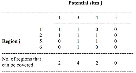
Figure 3. Sub-covering coefficient matrix after deleting Site 2
Step 5: Set the size of the population to the number of customers (m) in the Chromosome matrix (Each row of the matrix is treated as a chromosome).
Step 6: Find the fitness values of each chromosome in the initial population.
Step 7: Crossover Operation Step 7.1: Perform crossover operation by taking two chromosomes in succession starting from the chromosome 1 for each of the following pairs of logical operators.
(a) Logic OR and Logic AND
(b) Odd shift before Logic OR and Logic AND
(c) Even shift before Logic OR and Logic AND
(d) Logic OR and odd shift before Logic OR
(e) Logic OR and even shift before Logic OR
(f) Logic AND and odd shift before Logic AND
(g) Logic AND and even shift before Logic AND
[For example, if the number of rows of the chromosome matrix is 10 and Logic OR and Logic AND crossover operations are to be carried out, the first five offspring will be due to Logic OR crossover operation and the last five offspring will be due to Logic AND crossover operation. One should note that the number of offspring after performing crossover operation using a pair of logic operators will always be equal to the number of rows of the chromosome matrix (m)].
Step 7.2 In each case of Step 7.1, for each of the infeasible offspring, perform “Care and Share” operation and obtain a feasible offspring. Then replace that infeasible offspring with the feasible offspring, which is constructed using the “Care and Share” operation.
Step 8: In each case [from (a) to (g))] of the previous step, for each offspring, find the fitness function value.
Step 9: Club all the offspring of all the cases from (a) to (g) and sort them in the ascending order of their fitness function values.
Step 10: Store the top most offspring of the clubbed population of Step 9 as the current best chromosome along with its fitness function value.
Step 11: Choose the top m offspring from the clubbed population of Step 9 and store them in the chromosome matrix CM(I,J), for I = 1, 2, 3, …, m and J = 1, 2, 3, …, n.
Step 12: Increment the iteration number by 1 (I = I + 1).
Step 13: If I ≤ N, then go to Step 7; else go to Step 14.
Step 14: Print the current best chromosome along with its fitness function value.
Also print the customers, which are covered by each potential site that is assigned with a facility.
Step 15: Stop.
5. GRASP Heuristc
In this section, another heuristic based on Greedy Randomized Adaptive Search Procedure (GRASP) for the total covering problem is presented. The GRASP is an iterative procedure, which has two phases, namely construction phase and local search phase. In the construction phase, a feasible solution is constructed by choosing the next element randomly from the Candidate List (CL) [19]. The candidate list contains only the best elements selected by greedy function.
The Candidate List technique makes it possible to obtain different solution in each of the iterations. Since the solutions generated by the GRASP construction phase are not guaranteed to be the local optimum, it is recommended to apply the local search phase, which is the second phase of the GRASP. In this paper, a greedy heuristic is applied for the local search phase. At the end of each GRASP iteration, the better solution is updated. The latest best solution becomes the final solution, when the given termination criterion is reached.
The steps of GRASP based heuristic to locate the minimum number of facilities to cover all the customers are presented below.
Steps of GRASP Based Heuristic
Step 1: Input the covering co-efficient matrix, which is a square matrix of size m.
Step 2: Set the candidate = Null Set.
Step 3: Use the following Greedy heuristic to find the feasible solutions and add it to the Candidate List (CL).
Step 3.1: Find the number of ones in each column j of the Matrix C.
Let it be CSj
Step 3.2: Select the column (site) with the maximum CSj for assigning Facility.
Store the selected site number in the array Q.
Store the elements in the column corresponding to the selected site of the matrix C in an array F.
Set the actual number of sites selected [kk] to 1 Step 3.3: If Maximum CSj = m, then go to Step 3.8; otherwise go to Step 3.4.
Step 3.4: For each unselected site j (for j not in the array Q), find the total number of customers covered by the sites in the array Q after it is tentatively included in that array Q. Let it be TCj.
Step 3.5: Find the maximum TCj values.
Step 3.6: If there is no tie for the maximum TCj, then select the site with maximum TCj and place it in the array Q.
Otherwise find the number of ones in the each of the columns of the matrix C, corresponding to the maximum TCj.
Then select the column with maximum number of ones among such columns and place it in the array Q.
Increment the actual number of sites selected by 1 (kk = kk + 1).
Step 3.7: If Maximum TCj = m, then go to Step 3.8; otherwise go to Step 3.4.
Step 3.8: Treat the array Q as the Candidate List CL.
Step 4: Select the lone member of the Candidate List (CL), Let it be M.
Step 5: Set I = 1.
Step 6: Set the criterion Index, k = 0.
Step 7: Randomly select the position from the member M of CL and change it from 0-1 or 1–0.
Step 8: If the solution is feasible, do the following, or else go to step 9.
Step 8.1: Evaluate the solution and count the number of ones in the solution.
Step 8.2: Add the solution to the Candidate List.
Step 8.3: Up date k = 1.
Step 9: I = I + 1.
Step 10: If I ≤ 10 then go to step 7, or else go to step 11.
Step 11: if k = 0 then go to step 14, or else go to step 12.
Step 12: Find best solution from the Candidate List and let it be M.
Step 13: Go to step 5.
Step 14: Print the lastly used best solution (M), between steps 5 to step 10.
Step 15: Stop.
6. Factorial Experiment
In this section, first, the performance of the GA based heuristic is compared with that of the GRASP based heuristic and then it is compared with that of a model.
6.1 Comparison of GA Based Heuristic and GRASP Based Heuristic
This section presents the experimentation to compare the performance in terms of solution (number of potential sites selected for assigning facilities) of the proposed GA based heuristic (Alg1) and the GRASP based heuristic (Alg2) through a factorial experiment by considering three factors, viz. Percentage Sparsity of the covering coefficient matrix (percentage of number of 1s), Problem Size and Algorithm. Let the percentage sparsity be the Factor A, the Problem Size be the Factor B and the Algorithm be the Factor C. The Factor A is assumed with 5 levels (treatments), which are viz. 16%, 18%, 20%, 22% and 24%. The Factor B is assumed with 6 levels (treatments), which are, viz. 30 × 30, 40 × 40, 50 × 50, 60 × 60, 70 × 70 and 80 × 80. The Factor C is assumed with 2 levels (treatments), which are viz. Alg1 and Alg2. For each experimental combination, 5 replications are assumed.
In this experiment, the covering coefficient matrix of each benchmark problem is a square matrix. This means that each customer location is treated as a potential site for locating facility.
The corresponding ANOVA model [20] is shown below.
Yijkl = μ + Ai + Bj + ABij + Ck + ACik + BCjk
+ ABCijk + eijkl
whereYijkl is the response (number of sites assigned with facilities) of the lth replication for the ith treatment of the Factor A, jth treatment of the Factor B and kth treatment of the Factor C.
μ is the overall mean of the response.
Ai is the effect on the response due to the ith treatment of the Factor A Bj is the effect on the response due to the jth treatment of the Factor B ABij is the effect on the response due to the ith treatment of the Factor A and the jth treatment of the Factor B Ck is the effect on the response due to the kth treatment of the Factor C ACik is the effect on the response due to the ith treatment of the Factor A and the kth treatment of the Factor C BCjk is the effect on the response due to the jth treatment of the Factor B and the kth treatment of the Factor C ABCijk is the effect on the response due to the ith treatment of the Factor A, jth treatment of the Factor B and kth treatment of the Factor C eijkl is the random error associated with the lth replication under the ith treatment of the Factor A, jth treatment of the Factor B and kth treatment of the Factor C The different hypotheses relating to this model are as listed below.
Factor A (Percentage Sparsity of Covering Coefficient matrix)
H0: There is no significant difference in terms of solution between different pairs of treatments of the Factor A (Percentage sparsity of covering coefficient matrix)
H1: There is significant difference in terms of solution between different pairs of treatments of the Factor A (Percentage sparsity of covering coefficient matrix)
Factor B (Problem Size)
H0: There is no significant difference in terms of solution between different pairs of treatments of the Factor B (Problem Size).
H1: There is significant difference in terms of solution between different pairs of treatments of the Factor B (Problem Size).
Factor C (Algorithm)
H0: There is no significant difference in terms of solution between the two treatments of Factor C (Algorithm).
H1: There is significant difference in terms of solution between the two treatments of the Factor C (Algorithm).
Interaction Components:
Factor A × Factor B: (ABij)
H0: There is no significant difference in terms of solution between the different pairs of interaction between Factor A and Factor B.
H1: There is significant difference in terms of solution between different pairs of interaction between Factor A and Factor B.
Factor A × Factor C: (ACik)
H0: There is no significant difference in terms of solution between the different pairs of interaction between Factor A and Factor C.
H1: There is significant difference in terms of solution between different pairs of interaction between Factor A and Factor C.
Factor B × Factor C: (BCjk)
H0: There is no significant difference in terms of solution between the different pairs of interaction between Factor B and Factor C.
H1: There is significant difference in terms of solution between different pairs of interaction between Factor B and Factor C.
Factor A × Factor B × Factor C: (ABCijk)
H0: There is no significant difference in terms of solution between the different pairs of interaction between Factor A, Factor B and Factor C.
H1: There is significant difference in terms of solution between different pairs of interaction between Factor A, Factor B and Factor C.
A factorial experiment as per the above design was carried out to find the minimum number of potential sites which are to be assigned facilities under each experimental combination and such results (minimum number of potential sites assigned with facilities to cover all the customers) are summarized in Table 5. The results of ANOVA for the given factorial experiment are summarized in Table 6" target="_self"> Table 6. From the Table 6, it is clear that all the calculated F ratios are greater than the respective table F values at a significance level of 5%, except the interaction components ABij and ABCijk. Our prime concern is to check the significance of the effect of the Factor C (algorithm) on the response variable. The calculated F value for the Factor C is 2991.611 as against the table F value of 3.84. Hence, the corresponding null hypothesis is to be rejected and its alternate hypothesis is to be accepted. This means that there is significant difference between the algorithms (Alg1 and Alg2) in terms of providing the minimum number of potential sites, which are assigned with facilities to cover all the customers. If we closely look at the values of the responses in Table 5, for each experimental combination, the solution provided by the Algorithm Alg1 is less than the solution provided by the Algorithm Alg2. The mean response of the Algorithm Alg1 is 6.81 and that of the Algorithm Alg2 is 15.79. By combining the above two facts, it is evident that the Algorithm Alg1 performs better than the Algorithm Alg2 in terms of providing solution, that is the minimum number of potential sites assigned with facilities to cover all the customers. This means that the GA based heuristic performs better than the GRASP based heuristic.
6.2 Comparison of GA Based Heuristic with Model
Since, the GA based heuristic performs better than GRASP based heuristic, next it is mandatory to check the performance of the GA based heuristic with that of the
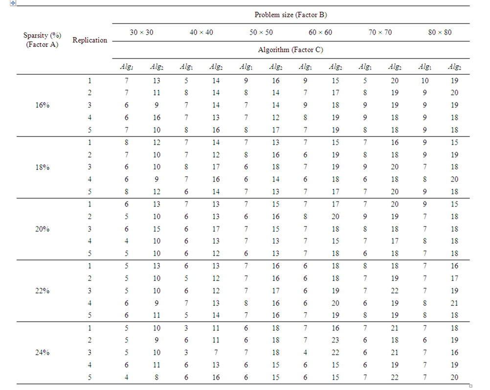
Table 5. Responses (minimum number of sites assigned with facilities) of factorial experiment for comparison of GA based heuristic and GRASP based heuristic
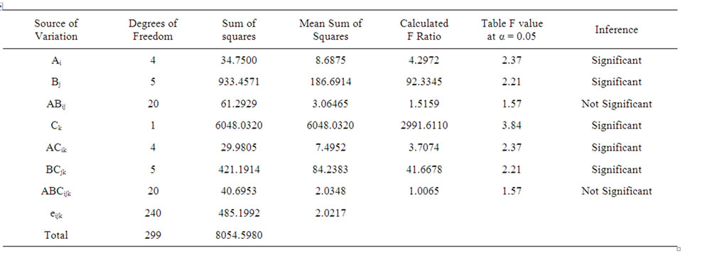
Table 6. ANOVA results for comparison of GA based heuristic with GRASP based heuristic
mathematical model as presented in Section 3, which gives the optimal solution. It is well known that solving any mathematical model will be limited by its number of variables and the number of constraints, because of the software which will be used to solve the problem of interest. So, in this section, problems of limited sizes, viz., 32 × 32, 34 × 34, 36 × 36, 38 × 38 and 40 × 40, each with five replications are considered for comparing the performance of the GA based heuristic (Method 1) and that of the model (Method 2). The Problem Sizes are assumed to be the levels of “Factor A” and the Methods are assumed to be the levels of “Factor B”.
The corresponding ANOVA model is shown below.
Yijk = μ + Ai + Bj + ABij + eijk
whereYijk is the response (number of sites assigned with facilities) of the kth replication for the ith treatment of the Factor A and the jth treatment of the Factor B.
μ is the overall mean of the response.
Ai is the effect on the response due to the ith treatment of the Factor A Bj is the effect on the response due to the jth treatment of the Factor B ABij is the effect on the response due to the ith treatment of the Factor A and the jth treatment of the Factor B eijk is the random error associated with the kth replication under the ith treatment of the Factor A and jth treatment of the Factor B.
The different hypotheses relating to this model are as listed below.
Factor A (Problem Size)
H0: There is no significant difference in terms of solution between different pairs of treatments of the Factor A (Problem Size).
H1: There is significant difference in terms of solution between different pairs of treatments of the Factor A (Problem Size).
Factor B (Method)
H0: There is no significant difference in terms of solution between different pairs of treatments of the Factor B (Method).
H1: There is significant difference in terms of solution between different pairs of treatments of the Factor B (Method).
Factor A × Factor B: (ABij)
H0: There is no significant difference in terms of solution between the different pairs of interaction between Factor A and Factor B.
H1: There is significant difference in terms of solution between different pairs of interaction between Factor A and Factor B.
A factorial experiment as per the above design was carried out to find the minimum number of potential sites which are to be assigned facilities under each experimental combination and such results (minimum number of potential sites assigned with facilities to cover all the customers) are summarized in Table 7. The results of ANOVA for the given factorial experiment are summarized in Table 8" target="_self"> Table 8. From the Table 8, it is clear that all the calculated F ratios are less than the respective table F values at a significance level of 5%. Our prime concern is to check the significance of the effect of the Factor B (Method) on the response variable. The calculated F value for the Factor B is 1.5283 as against the table F value of 4.09. Hence, the corresponding null hypothesis is to be accepted and its alternate hypothesis is to be rejected. This means that there is no significant difference between the methods (Method 1 and Method 2) in terms of providing the minimum number of potential sites, which are assigned with facilities to cover all the customers. So, the performance of the GA based heuristic is equivalent to that of the model for the assumed problems of limited sizes.
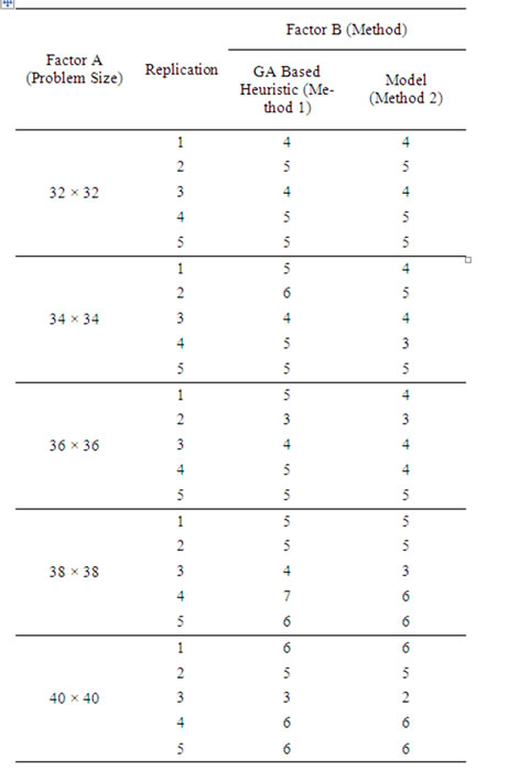
Table 7. Results of GA based heuristic and model
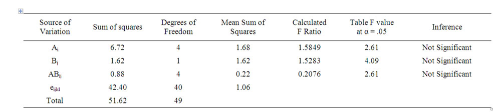
Table 8. ANOVA results of comparison of GA based heuristic and model
7. Conclusions
The total covering problem under facility location problem is an important problem to determine the minimum number of sites to locate the facilities to cover all the customers. Since, this problem comes under combinatorial category, in this paper, an attempt has been made to develop heuristics and compare them in terms of their performance. In the first phase, the design of GA based heuristic is given and it is followed by the design of GRASP based heuristic. Later, a complete factorial experiment has been conducted to compare the performance of the two heuristics by assuming three factors, Factor A (Percentage Sparsity), Factor B (Problem Size) and Factor C (Algorithms). The Factor A is assumed with 5 levels, which are viz. 16%, 18%, 20%, 22% and 24%. The Factor B is assumed with 6 levels, which are, viz. 30 × 30, 40 × 40, 50 × 50, 60 × 60, 70 × 70 and 80 × 80. The Factor C is assumed with 2 levels, which are viz. Alg1 and Alg2. For each experimental combination, 5 replications are carried out. Through ANOVA, it is found that the GA based heuristic performs better than the GRASP based heuristic in terms of providing the solution for the total covering problem.
After having concluded that the GA based heuristic performs better than the other heuristic, in the next phase, a comparison is done between the solution of the GA based heuristic and that of the mathematical model presented in Section 3 for the total covering problem through a two factor complete factorial experiment. In this experiment five different problem sizes (32 × 32, 34 × 34, 36 × 36, 38 × 38 and 40 × 40) are considered. For each problem size, five replications are considered. By taking the problem size as one factor and the methods of solving the total covering problem (GA based heuristic and Model) as another factor, a factorial experiment was conducted and found that the there is no difference between the methods, viz., GA based heuristic and model in terms of providing solution for the total covering problem. Hence, it is concluded that the performance of the GA based heuristic can be equated to that of the model which gives optimal solution for small and moderate size problems. The reason of limiting the problem size to a maximum of 40 × 40 in this comparison is due the limitations of the number of variables and the number of constraints of a model that can be handled by software. Finally, it is concluded that the GA based heuristic performs better than the GRASP based heuristic to solve the total covering problem. Further, there is no significant difference between the GA based heuristic and the mathematical model, in terms of providing solution for the total covering problem for moderate size problems.
REFERENCES
- R. Panneerselvam, “Production and Operations Management,” 2nd Edition, Prentice-Hall India (P) Ltd., New Delhi, 2005.
- C. Toregas, R. Swain, C. Revelle and L. Bergman, “The Location of Emergency Service Facilities,” Operations Research, vol. 19, No. 6, 1971, pp. 1363-1373.
- N. R. Patel, “Location of Rural Social Service Centers in India,” Management Science, vol. 25, no. 1, 1979, pp. 22-30.
- T. D. Klastorin, “On the Maximal Covering Location Problem and the Generalized Assignment Problem,” Management Science, vol. 25, no.1, 1979, pp. 107-111.
- O. Saatcioglu, “Mathematical Programming Model for Airport Site Selection,” Transportation Research-B, vol. 16B, no. 6, 1982, pp. 435-447.
- A. W. Neebe, “A Procedure for Locating EmergencyService Facilities for All Possible Response Distances,” Journal of Operational Research Society, vol. 39, no. 8, 1988, pp. 743-748.
- R. Panneerselvam, “A Heuristic Algorithm for Total Covering Problem,” Industrial Engineering Journal, vol. 19, no. 2, 1990, pp. 1-10.
- G. Rajkumar and R. Panneerselvam, “An Improved Heuristic for Total Covering Problem,” Industrial Engineering Journal, vol. 20, no. 8, 1991, pp. 4-7.
- R. Panneerselvam, “Efficient Heuristic for Total Covering Problem,” Productivity, vol. 36, no. 4, 1996, pp. 649- 657.
- M. E. O’Kelly, “The Location of Interacting Hub Facilities,” Transportation Science, vol.20, no.2, 1986, pp. 92- 106.
- T. B. Boffey, “Location Problems Arising in Computer Networks,” Journal of Operational Research Society, vol. 40, no. 4, 1989, pp. 347-354.
- T. J. Chen and C. A. Yano, “A Multiplier Adjustment Approach for Set Partitioning Problem,” Operations Research, vol. 40, no. 1, 1992, pp. 40-47.
- W. A. Chaovalitwongse, T. Y. Berger-Wolf, B. Dasgupta and M. V. Ashley, “Set Covering Approach for Reconstruction of Sibling Relationships,” Optimization methods and software, vol. 22, no. 1, 2007, pp. 11-24.
- B. Pelegrin, J. L. Redondo, P. Fernandez, I. Garcia and P. M. Ortigosa, “GASUB: Finding Global Optima to Discrete Location Problems Genetic—Like Algorithm,” Journal of Global Optimization, vol. 38, no. 2, 2007, pp. 249-264.
- Sibel A. Alumur, Bahar Y. Kara and Oya E. Karasan, “The Design of Single Allocation in Complete Hub Networks,” Transportation Research B: Methodological, vol. 43, no. 10, 2009, pp. 936-951.
- V. Marianov, M. Mizumori and C. Re Velle, “The Heuristic Concentration—Integer and its Application to a Class of Location Problems,” Computers and Operations Research, vol. 36, no. 5, 2009, pp. 1406-1422.
- De A. C. Francisco, N. L. L. Antonio and M. R. Glaydston, “A Decomposition Approach for the Probabilistic Maximal Covering Location—Allocation Problem”, Computers and Operations Research, vol. 36, no. 10, 2009, pp. 2729-2739.
- V. Batanovic, D. Petrovic and R. Petrovic, “Fuzzy Logic Based Algorithms for Maximum Covering Location Problems,” Information Sciences, vol. 179, no. 1-2, 2009, pp. 120-129.
- T. A. Feo and M. G. C. Resende, “Greedy Randomized Adaptive Search Procedures,” Journal of Global Optimization, vol. 6, 1995, pp. 109-133.
- R. Panneerselvam, “Research Methodology,” PrenticeHall India (P) Ltd., New Delhi, 2004.