Natural Science
Vol.5 No.1A(2013), Article ID:27622,7 pages DOI:10.4236/ns.2013.51A023
Time-integrated North Atlantic Oscillation as a proxy for climatic change
![]()
Meteorological Observatory, Department of Science of the Earth, Environment and Resources, University of Naples “Federico” II, Naples, Italy; adriano.mazzarella@unina.it
Received 28 November 2012; revised 30 December 2012; accepted 12 January 2013
Keywords: North Atlantic Oscillation (NAO); Length of Day (LOD); Sea Surface Temperature (SST); Correlation Coefficient; Vector Probable Error
ABSTRACT
The time-integrated yearly values of North Atlantic Oscillation (INAO) are found to be well correlated to the sea surface temperature. The results give the feasibility of using INAO as a good proxy for climate change and contribute to a more complete picture of the full range of variability inherent in the climate system. Moreover, the extrapolation in the future of the well identified 65-year harmonic in INAO suggests a gradual decline in global warming starting from 2005.
1. INTRODUCTION
Forecasting of climatic changes is usually performed by general circulation models (GCM) that utilize the fundamental principles of physics. However, the results are controversial because GCM approximate solutions through the numerical integration of the equations and parameterize all processes that occur on spatial scales smaller than the distance between network points. A large portion of public opinion and a part of scientific community is persuaded that all the results obtained by GCMs must be accepted “fide et amore dei” just because these computer models have implemented in their codes a set of known mathematical-physical laws discovered via proper lab-experiments. But, the climate is a complex system and cannot be tested not reproduced in a controlled lab experiment. As the science of complexity points out, the mere accuracy of the fundamental physical laws of nature does not guarantee the scientific accuracy of every mathematical model attempting to combine them to reproduce the behaviour of a macroscopic complex system [1]: although the fundamental physical laws are tested in controlled lab-experiments, their mutual coupling and interconnection mechanisms, which are required for reproducing a macroscopic complex system, are not. This kind of methodological problems are well known and understood in many scientific disciplines dealing with complex natural system, such as in biology and medicine (see for example a nice comment by [2]). Curry and Webster [3] have recently warned about the monstrous uncertainty implicit in the current analytical climate modelling approach, which has been interpreted as due to model inadequacy, uncertainty in model parameter values, and initial condition uncertainty. Recently, a phenomenological and unitary approach in which the length of day (LOD) is considered as the integral of the different circulations that occur within the ocean-atmosphere system both along latitude (zonal circulation) and longitude (meridional circulation) has been set up [4-6]. Such an approach has allowed identification of a good relationship between LOD and sea surface temperature (SST) and its forecast 4 years in advance. The North Atlantic Oscillation (NAO) is the main synoptic mode of atmospheric circulation and climate variability in the North Atlantic/European sector and has a substantial influence on marine-terrestrial ecosystems and regional socio-economic activity. To compare the forecasting reliability of NAO and LOD, we integrate NAO yearly values into INAO yearly data according to a sequential summation of values of NAO. INAO yearly data have been calculated in such a way that they are directly proportional to a zonal wind speed and inversely proportional to LOD. Herein we will show that the INAO yearly values can be used as a more reliable proxy for Northern hemisphere air/sea temperature than LOD. Moreover, the clear identification of the 65-yr cycle in INAO and the extrapolation of such a cycle in the future suggests a gradual decline in global warming starting from 2005.
2. COLLECTION OF DATA
We analyze the historical series of:
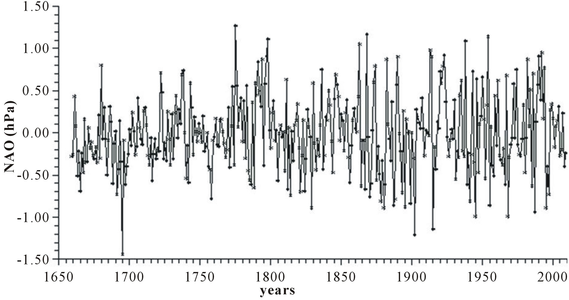
1) North Atlantic Oscillation (NAO) (hPa) defined as the normalized sea level pressure between the Azores high and Icelandic low [7-9] (interval, 1861-2011). Because the shortness of the available instrumental records, we use the series of yearly NAO values as reconstructed by Lutherbacher et al. [10] who utilized instrumental and documentary proxy data to extend NAO back to 1659.
The yearly data of NAO are taken from the web site:
ftp://ftp.ncdc.noaa.gov/pub/data/paleo/historical/north_atlantic/nao_mon.txt and reported in Figure 1(a).
The prevailing regional flow can be derived easily from just the sign an the magnitude of each index. To obtain a cumulative effect of NAO, we integrate NAO yearly values into an integrated NAO (INAO) annual record according to a sequential summation of NAO, for each year “t”, i.e.,
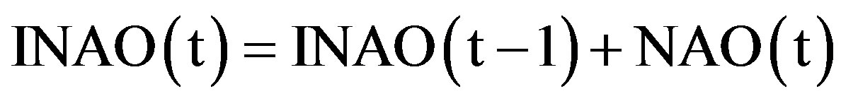
Figure 1(d) depicts INAO yearly series.
2) The Earth’s rotation speed as normally measured by means of LOD (ms). This record represents the difference between the astronomical LOD and the standard length (interval: 1657-2011) [11]. The LOD yearly data are taken from the web site: http://www.iers.org/iers/earth/rotation/ut1LOD/table3.html and reported in Figure 1(b).
3) Sea surface temperature SST (˚C) provided by the Climatic Research Unit, University of East Anglia (interval: 1850-2011) [12,13]. Owing to the very large thermal capacity of the ocean, SST behaves like a natural filter that eliminates all the short-term variations that normally affect air temperature that is measured on land stations often biased by the environment in which they operate. The analysis here is confined to the Northern Hemisphere since our aim is to investigate the potential relationship between INAO and SST. The yearly data of the Northern Hemisphere SST are available from the website: http://www.cru.uea.ac.uk/cru/data/temperature/ and reported in Figure 1(c).
3. ANALYSIS
Circulation indices such as zonal and meridional indices are used very frequently to define regional circulation [14]. These indices are defined as the difference in atmospheric pressure at the same level, between two regions located at different latitudes or longitudes. Their greatest advantage is that they integrate all the complex distribution of pressures over an entire region into a single figure, thus enabling an easier comparison between various situations. Here we investigate the NAO index that is the main synoptic mode of atmospheric circulation and climate variability in the North Atlantic/European sector. NAO (hPa) index is a gradient of atmospheric pressure between the Azores high and Icelandic low [7- 9]. LOD has been already verified to be a good proxy for climatic changes [4-6] and here we will investigate also
 (a)
(a)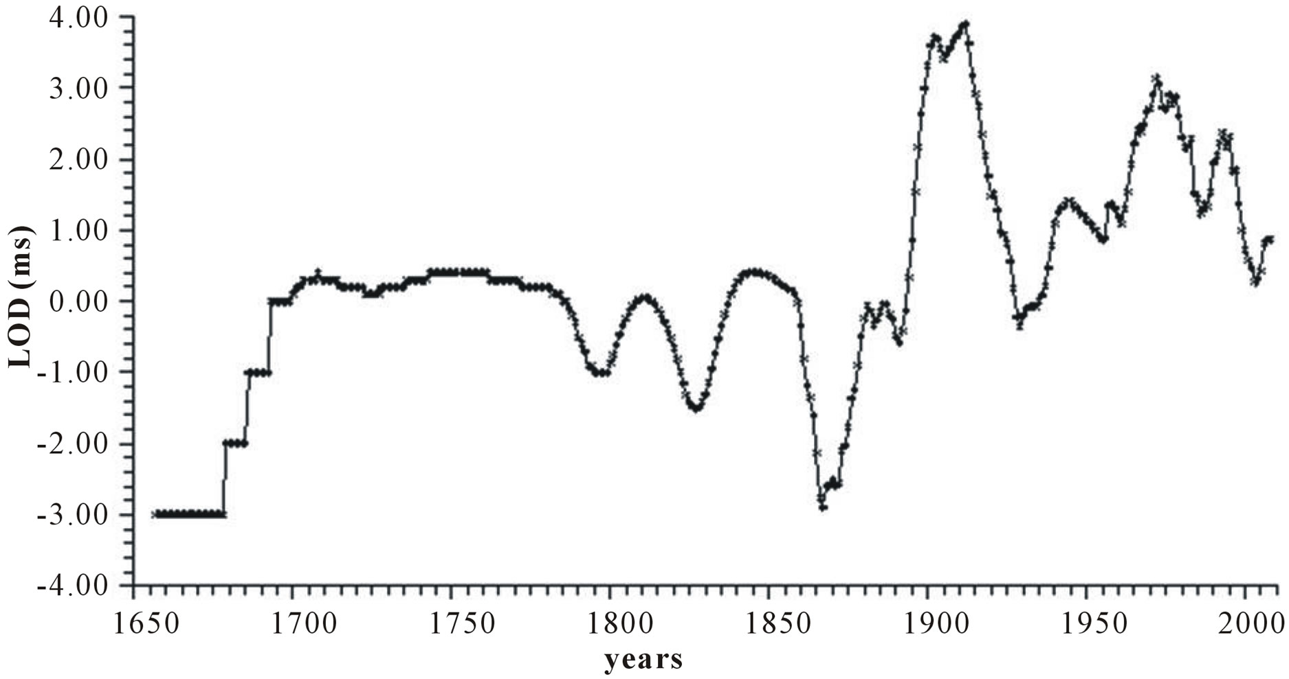 (b)
(b)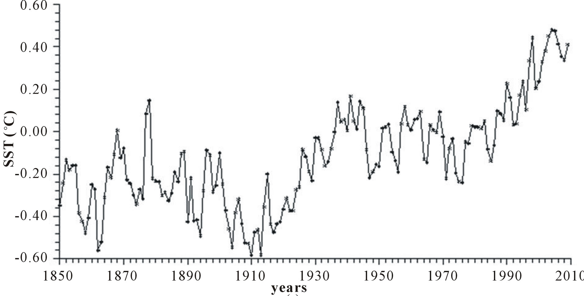 (c)
(c)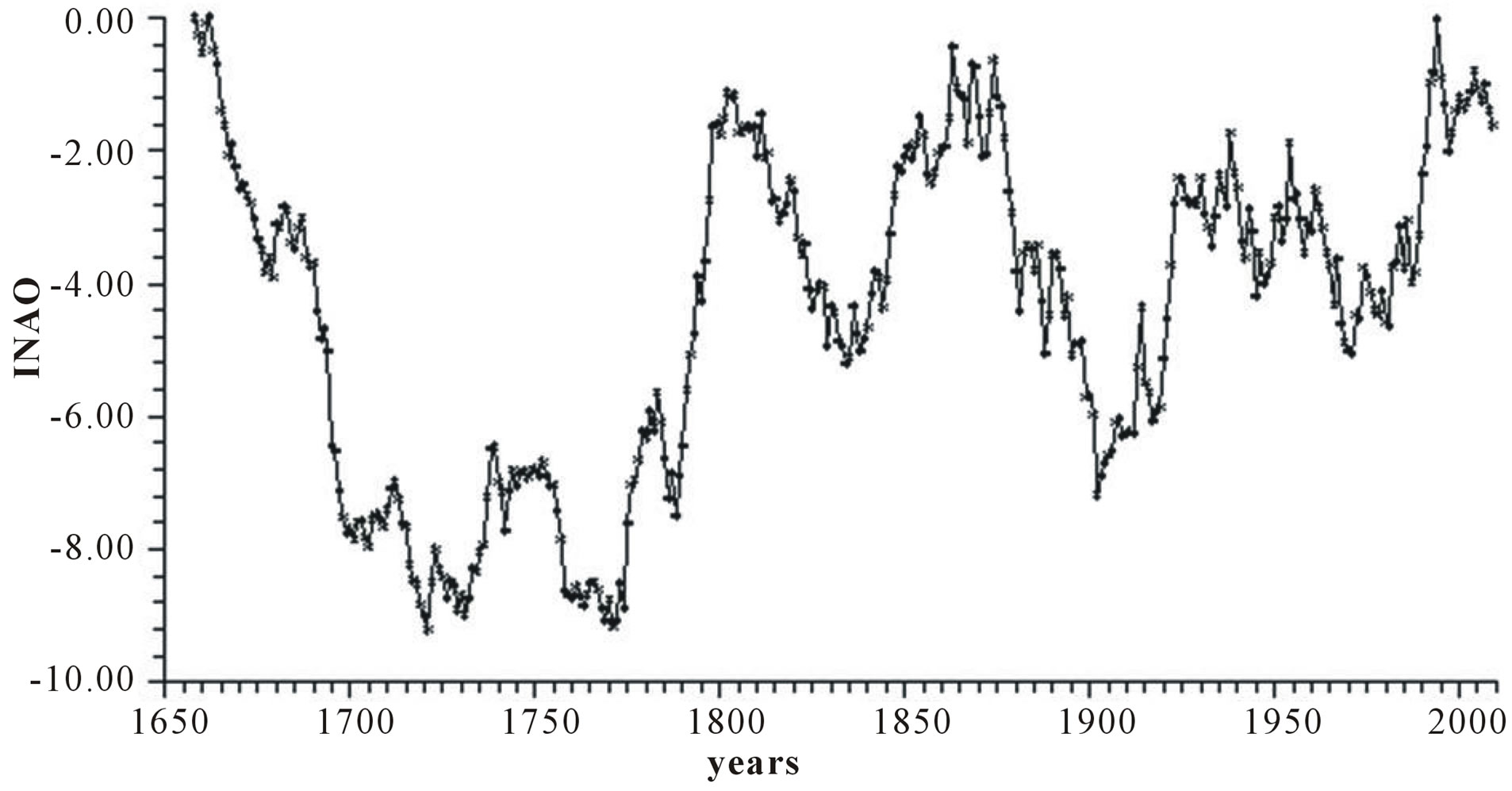 (d)
(d)
Figure 1. Time plot of yearly values of: (a) North Atlantic Oscillation NAO (hPa); (b) Length of day LOD; (c) Sea surface temperature SST; (d) Integrated NAO oscillation INAO.
NAO as proxy for climatic changes. To compare the forecasting reliability of NAO and LOD, we integrate NAO yearly values into INAO yearly data according to a sequential summation of yearly values of NAO. INAO yearly data have been calculated in such a way that they are directly proportional to a zonal wind speed and inversely proportional to LOD. Both the series are reported in Figures 1(a) and (d). Finally, for visual inspection, we normalize all the subsequent plots to a mean equal to zero and to a standard deviation equal to one.
3.1. Running Mean Method
The running mean method is equivalent to a low pass filtering with no change in amplitude and phase [15] and helps remove all the oscillations with periods shorter than the order of the running mean. Here, to eliminate the modulation of solar activity and to remove all the oscillations with periods shorter than 5, 11, 23 year, a running mean of order 5, 11, 23, respectively, is used. Such a methodology provides a more accurate low frequency spectral analysis of the investigated series than when they are biased by high-frequency waves and by noncyclic variation.
3.2. Correlation Coefficient
To investigate whether or not two random variables are interrelated, we here use the correlation coefficient R [15] whose square represents the fractional portion of the variance of the N values of one series explained by the other one. Since we are interested in the physical reality of the relationship between each pair of investigated variables, particular attention is paid here to their reliability. So, to evaluate the accuracy of R, we compute the random variable 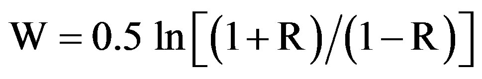 [15]. The level of confidence of R is obtained by testing W (normalized to a mean equal to zero and to a variance equal to one) versus the null hypothesis of zero population relationship according to the standard one-sided z test. The correlation coefficient is found to be confident at 95% (99%) level when the relationship:
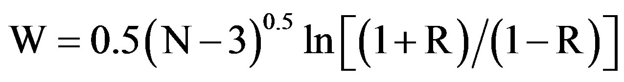
provides values ≥ 1.96 (≥2.58).
3.3. Vector Probable Error
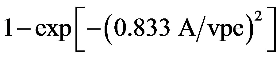
To obtain a more detailed information on the harmonics constituting a time series, we follow the vector probable statistics [15,16]. The method subdivides the entire observation interval into non overlapping subintervals (with a length equal to the period of the harmonic to be investigated). The approach consists in the calculation of the Fourier coefficients for each of the subintervals and of the scattering of the individual harmonics from the center of gravity A of all points. This corresponds to the harmonic coefficients as computed from all series and so to the amplitude of the investigated harmonic. The reliability is computed according to the vector probable error (vpe) equal to the root-mean square radius of the point cloud. The confidence level of the harmonic is computed according to the equation:
 .
.
The harmonic is found to be confident at 95% (99%) level when A ≥ 2.08 vpe (A ≥ 3.00 vpe). The method is iterative and must be performed for all possible subintervals. Finally one considers the highest value of A/vpe ratio and computes its reliability.
4. RESULTS
4.1. Time Domain
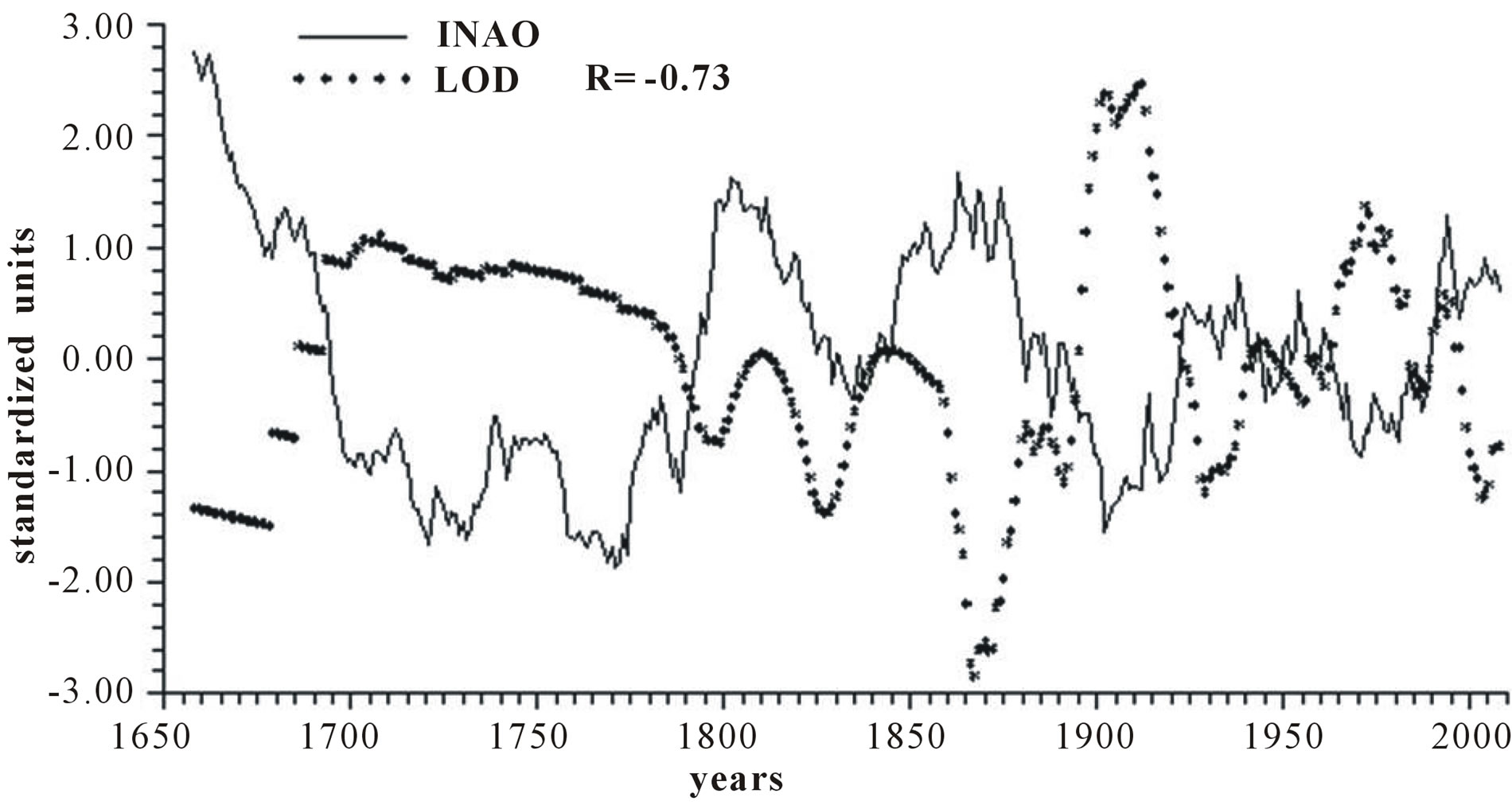
Figure 2 reports the time plots of raw yearly values of INAO and LOD and smoothed according to 5-yr, 11-yr and 23-yr running means together with the relative correlation coefficient “R”. It appears that INAO is inversely related to LOD with a correlation coefficient gradually increasing from −0.73, to −0.74, to −0.77 and to −0.82, indicating that an increase in zonal wind speed is responsible for an ever more effective decrease in LOD as the time scale increases.
Figure 3 reports the time plots of raw yearly values of LOD and SST and smoothed according to 5-yr, 11-yr and 23-yr running means together with the relative correlation coefficient “R”. It appears that LOD is inversely related to SST, with a peak in the relationship when LOD is shifted ahead by 4 years, with a correlation coefficient gradually increasing from −0.66, to −0.79, to −0.89 and to −0.96, indicating that an increase in LOD is responsible for an ever more effective increase in SST as the time scale increases.
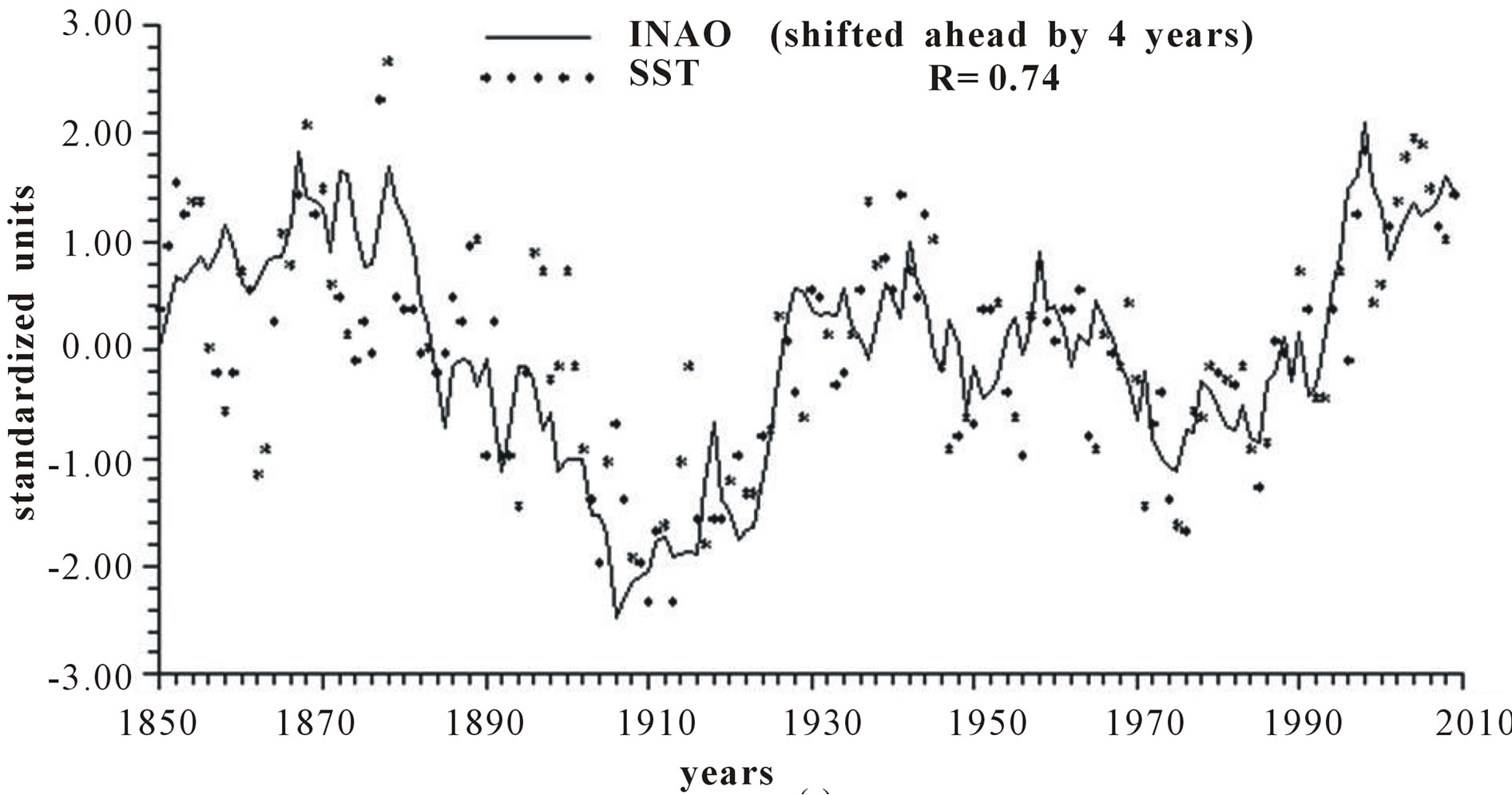
Figure 4 reports the time plots of raw yearly values of INAO and SST and smoothed according to 5-yr, 11-yr and 23-yr running means together with the relative correlation coefficient “R”.
4.2. Frequency Domain
To investigate whether INAO can be reasonably considered as a proxy for climatic changes, we must obtain a more detailed information on the dominant harmonics constituting INAO yearly series and for this we follow the vector probable statistics [16]. After several trials, we have found that a confidence level greater than 99% is obtained only when we subdivide the 23-yr running mean INAO series into subintervals of 65 years. The A/vpe ratio is found to reach the highest value of 9.3 and this corresponds to an identification of 65-yr harmonic with a confidence level greater than 99%. Such a harmonic is found to account for more than 25% of the total yearly INAO variability. The amplitude (A) and phase (f) of the identified 65-year INAO harmonic are found to be
 (a)
(a)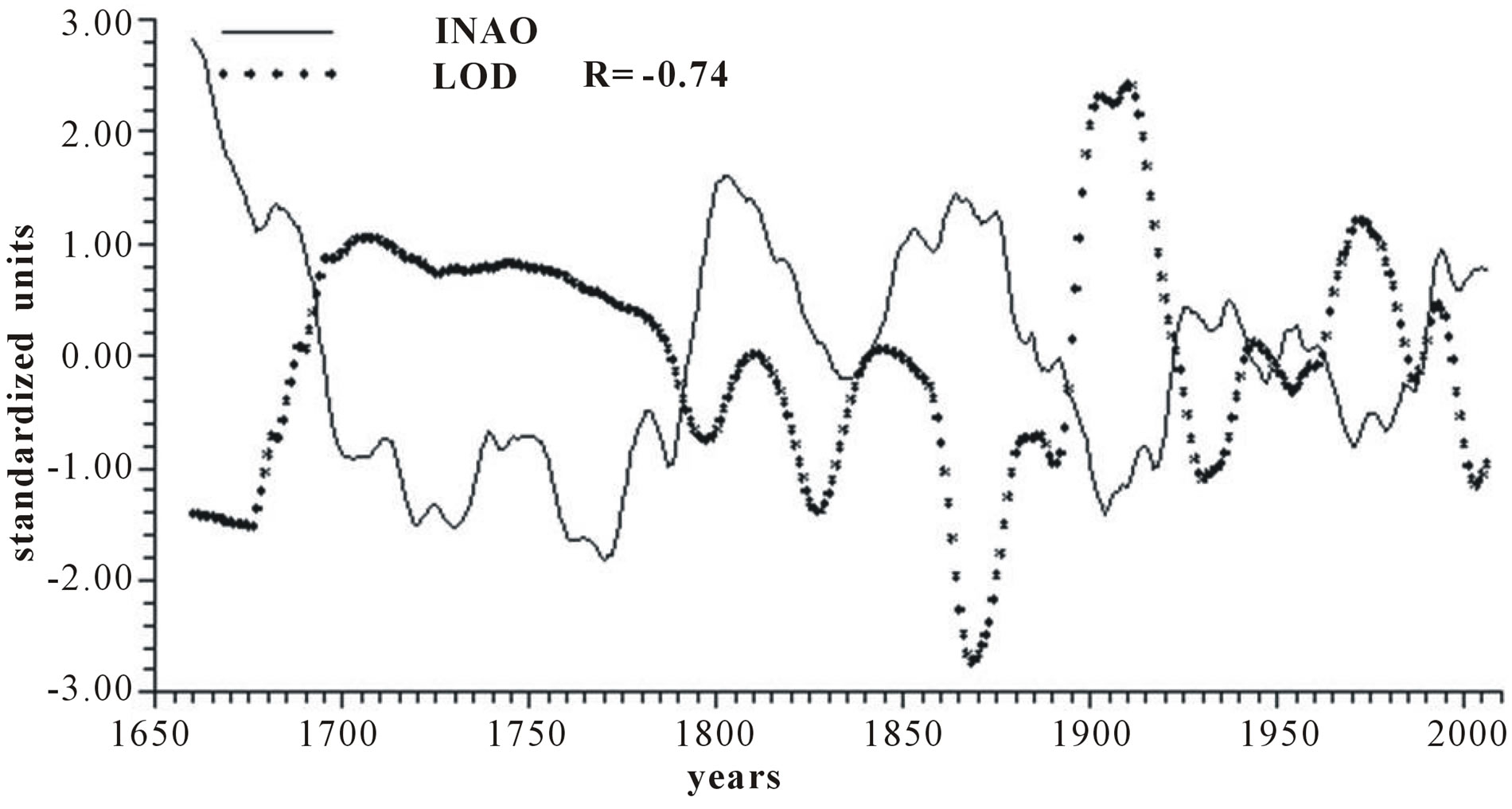 (b)
(b)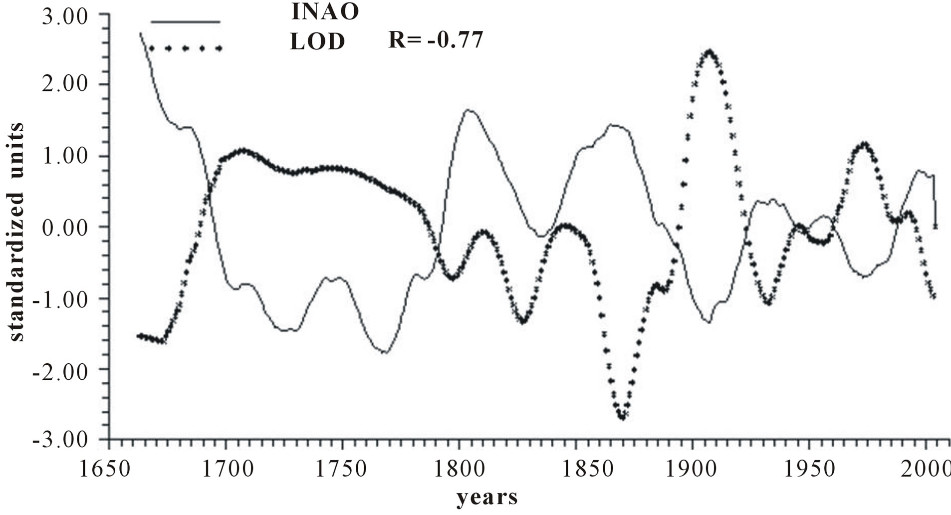 (c)
(c)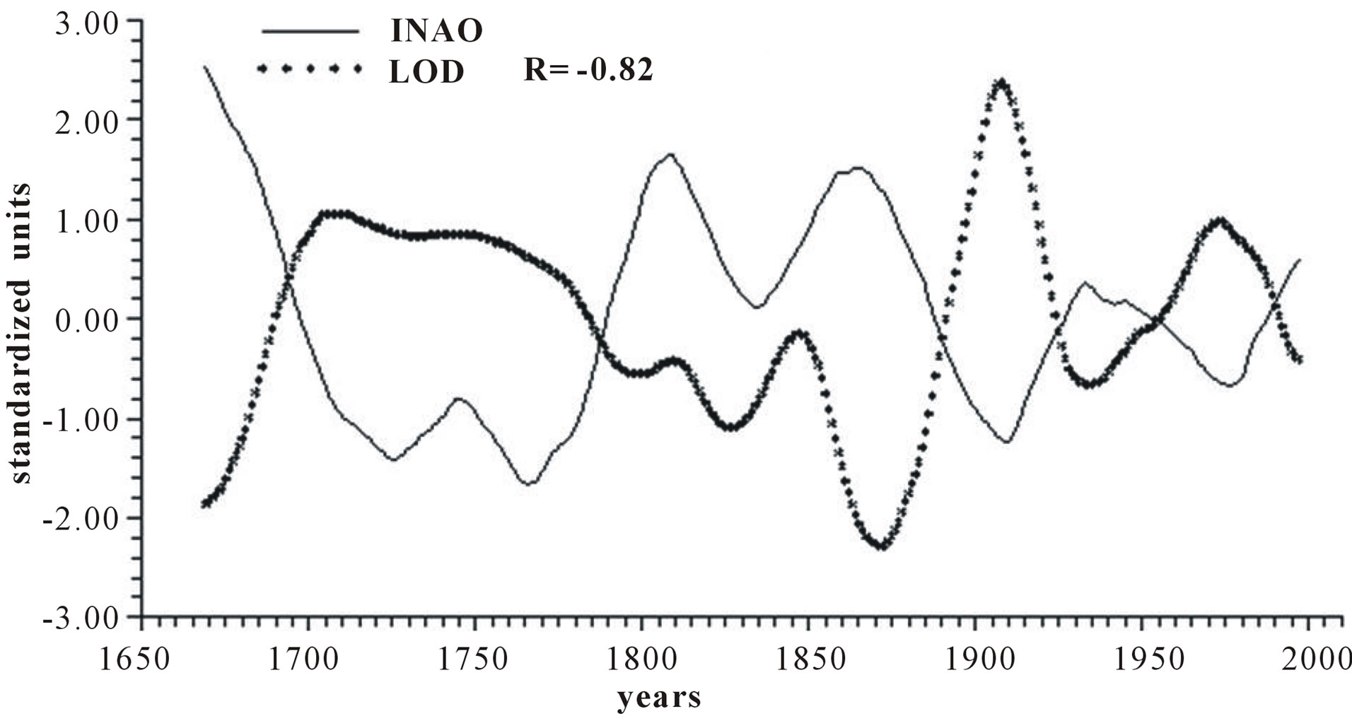 (d)
(d)
Figure 2. Time plot of detrended yearly values of INAO and LOD: (a) Raw values; (b) Smoothed according to a 5-yr running mean; (c) Smoothed according to a 11-yr running mean; (d) Smoothed according to a 23-yr running mean.
equal to: 1.24, 50.8˚. Thus, we may forecast the value of INAO at any year “t” ahead until 2060 by introduction the time t into the equation
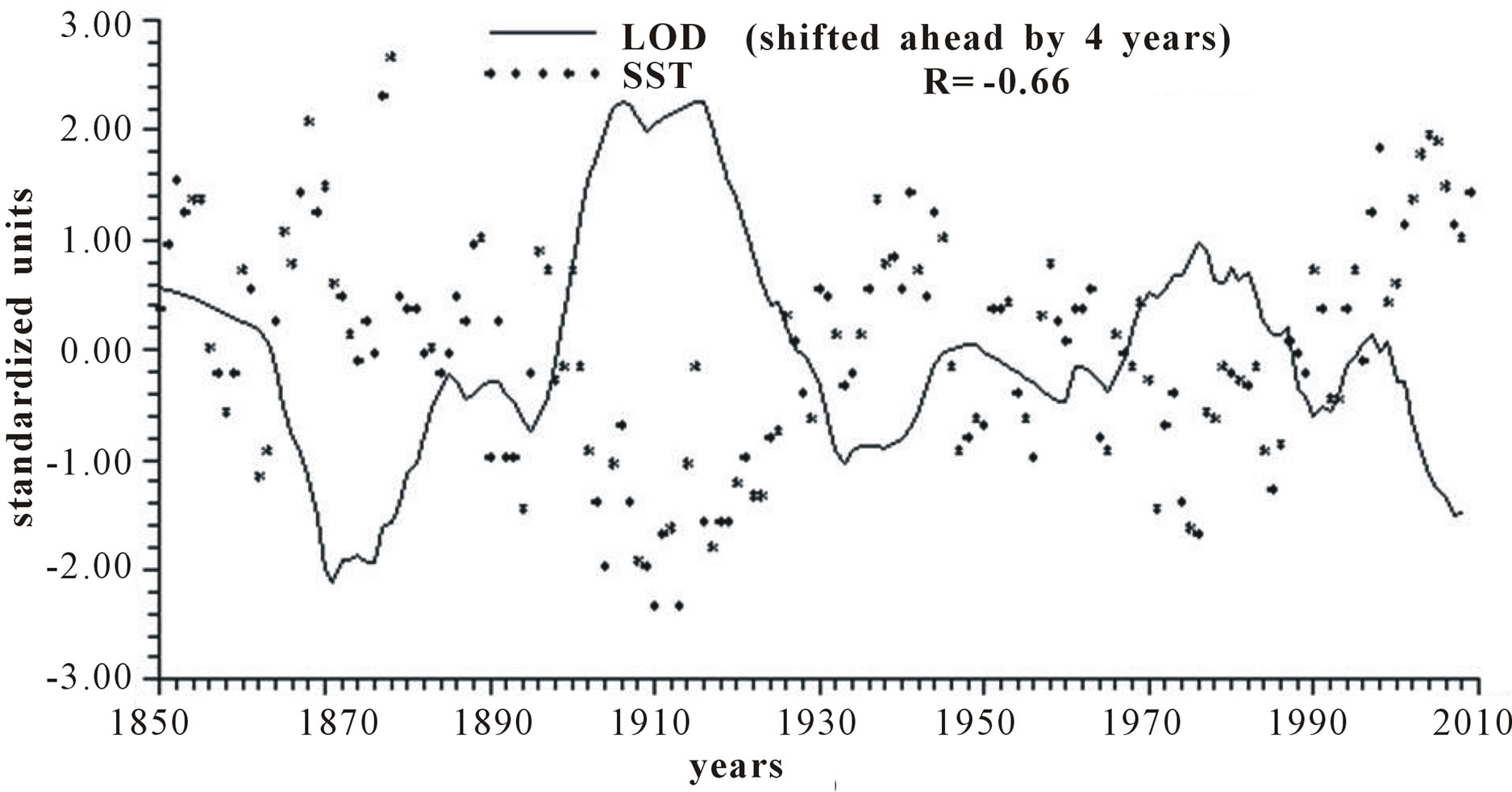 (a)
(a)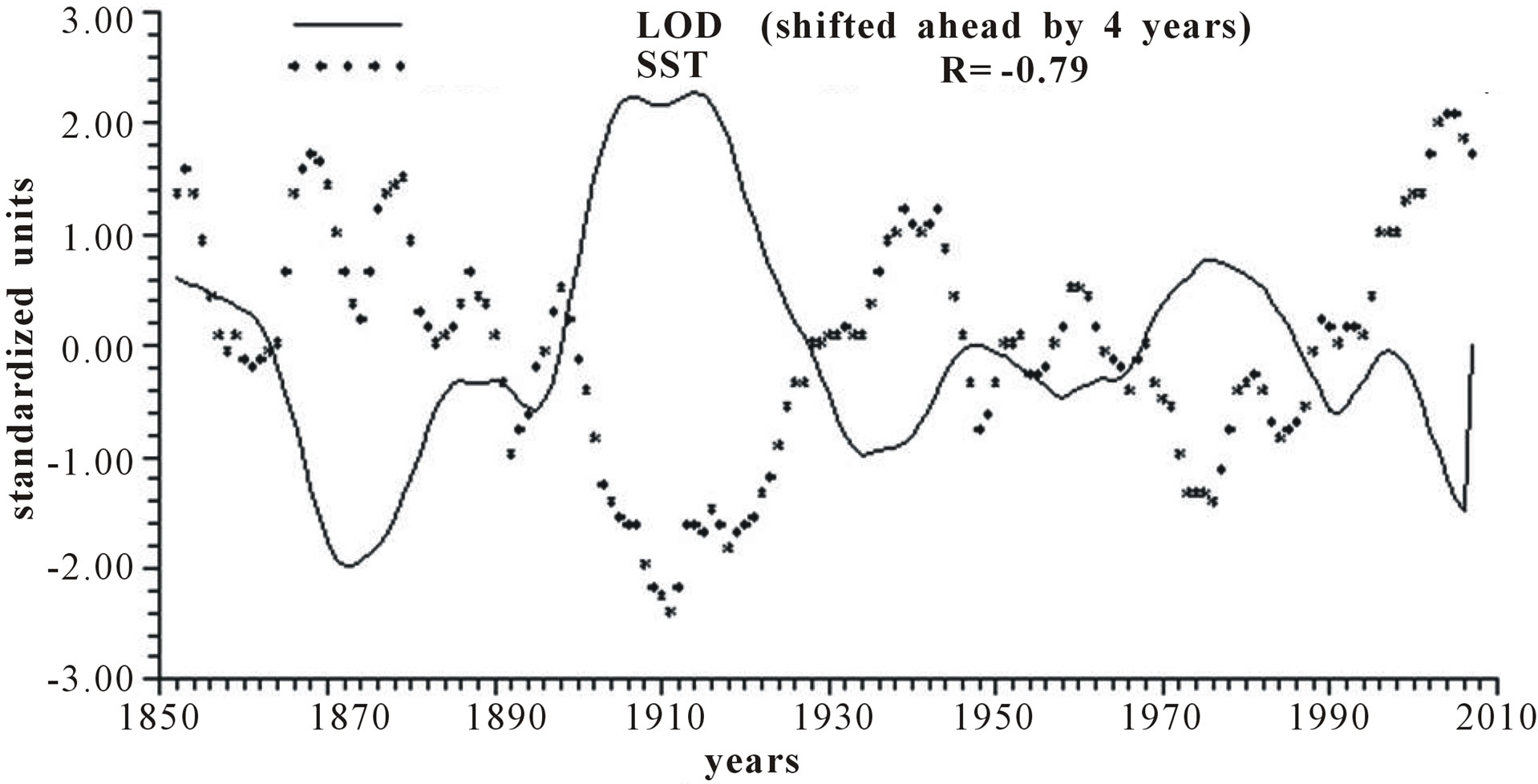 (b)
(b)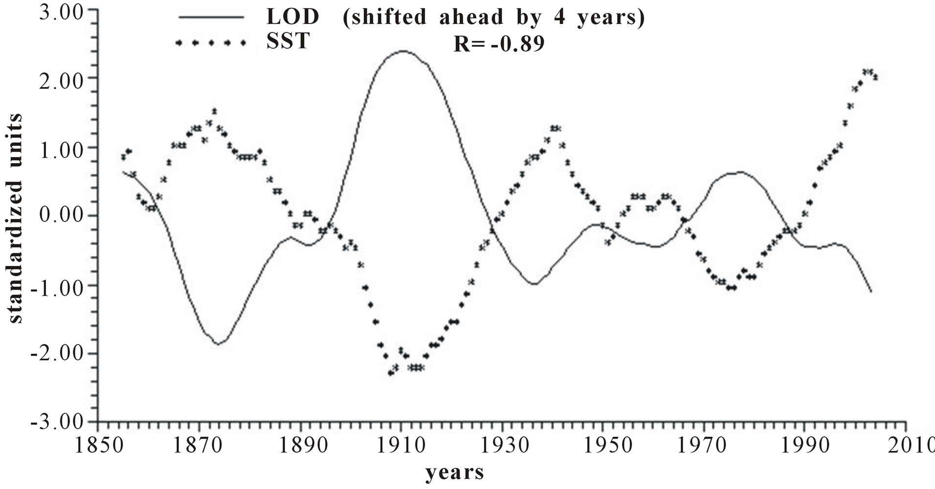 (c)
(c)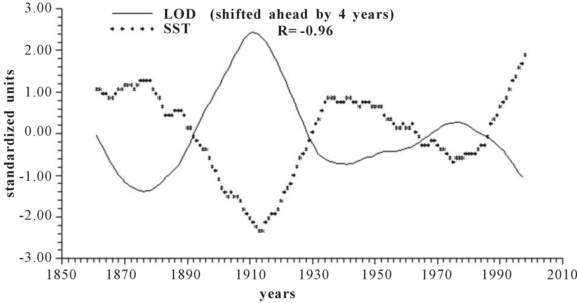 (d)
(d)
Figure 3. Time plot of detrended yearly values of LOD and SST: (a) Raw values; (b) Smoothed according to a 5-yr running mean; (c) Smoothed according to a 11-yr running mean; (d) Smoothed according to a 23-yr running mean.
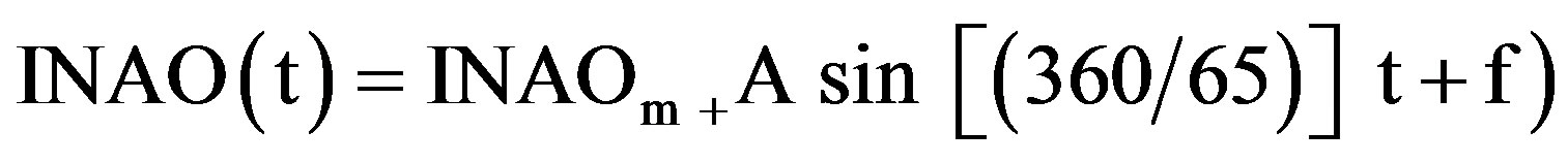 .
.
where INAOm is the mean value of INAO and A and f represent the amplitude and the phase of the 65-yr har-
 (a)
(a)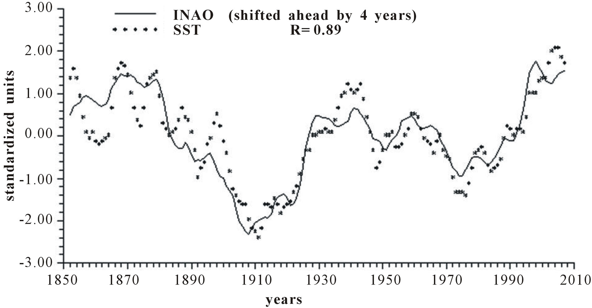 (b)
(b)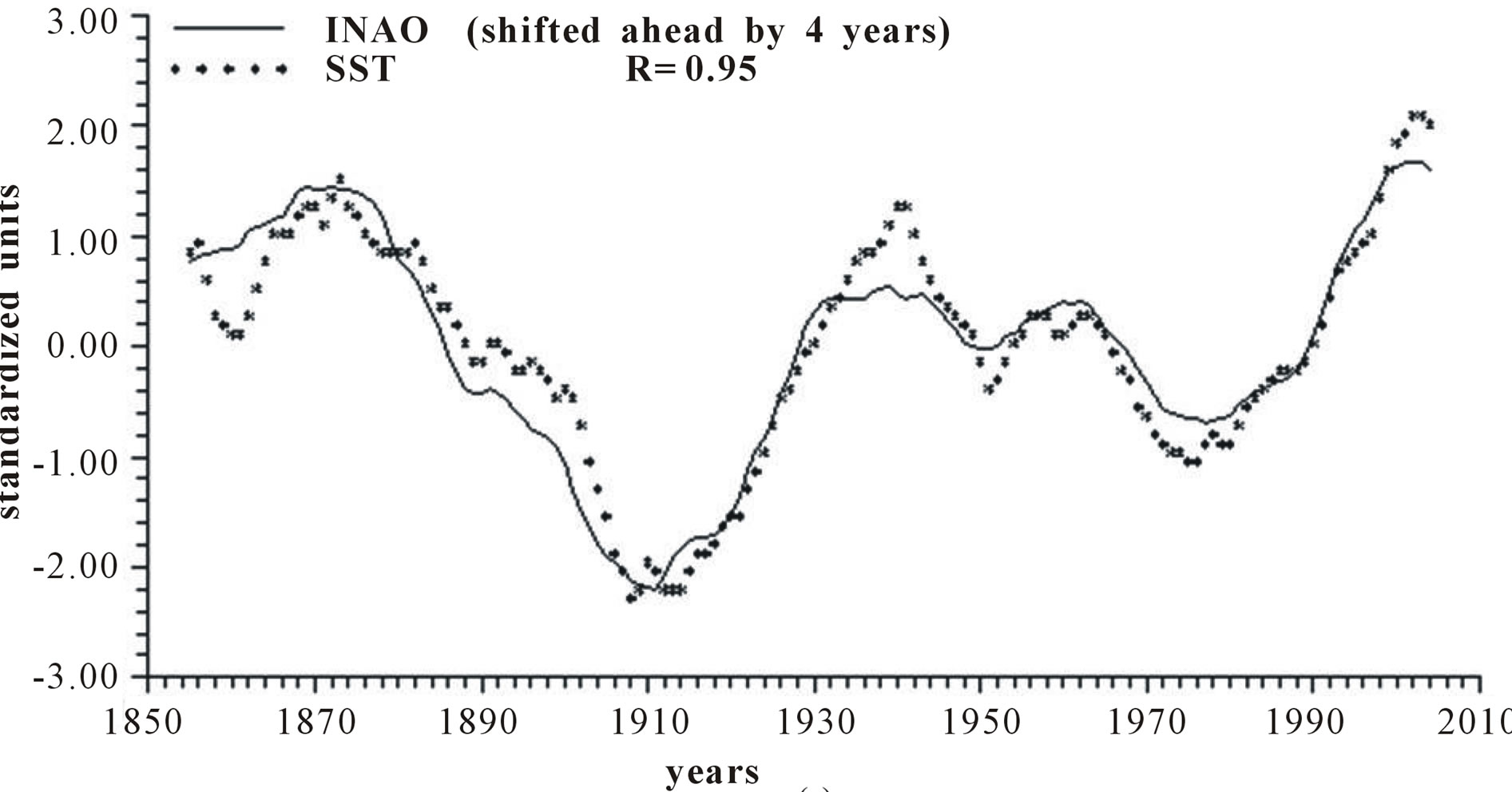 (c)
(c)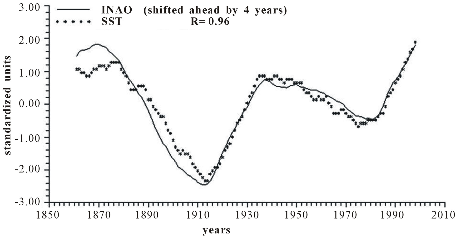 (d)
(d)
Figure 4. Time plot of detrended yearly values of INAO and SST: (a) Raw values; (b) Smoothed according to a 5-yr running mean; (c) Smoothed according to a 11-yr running mean; (d) Smoothed according to a 23-yr running mean.
monic respectively.
Figure 5 depicts the time plot of 23-yr running mean of INAO and of its 65-yr harmonic extrapolated until 2060.
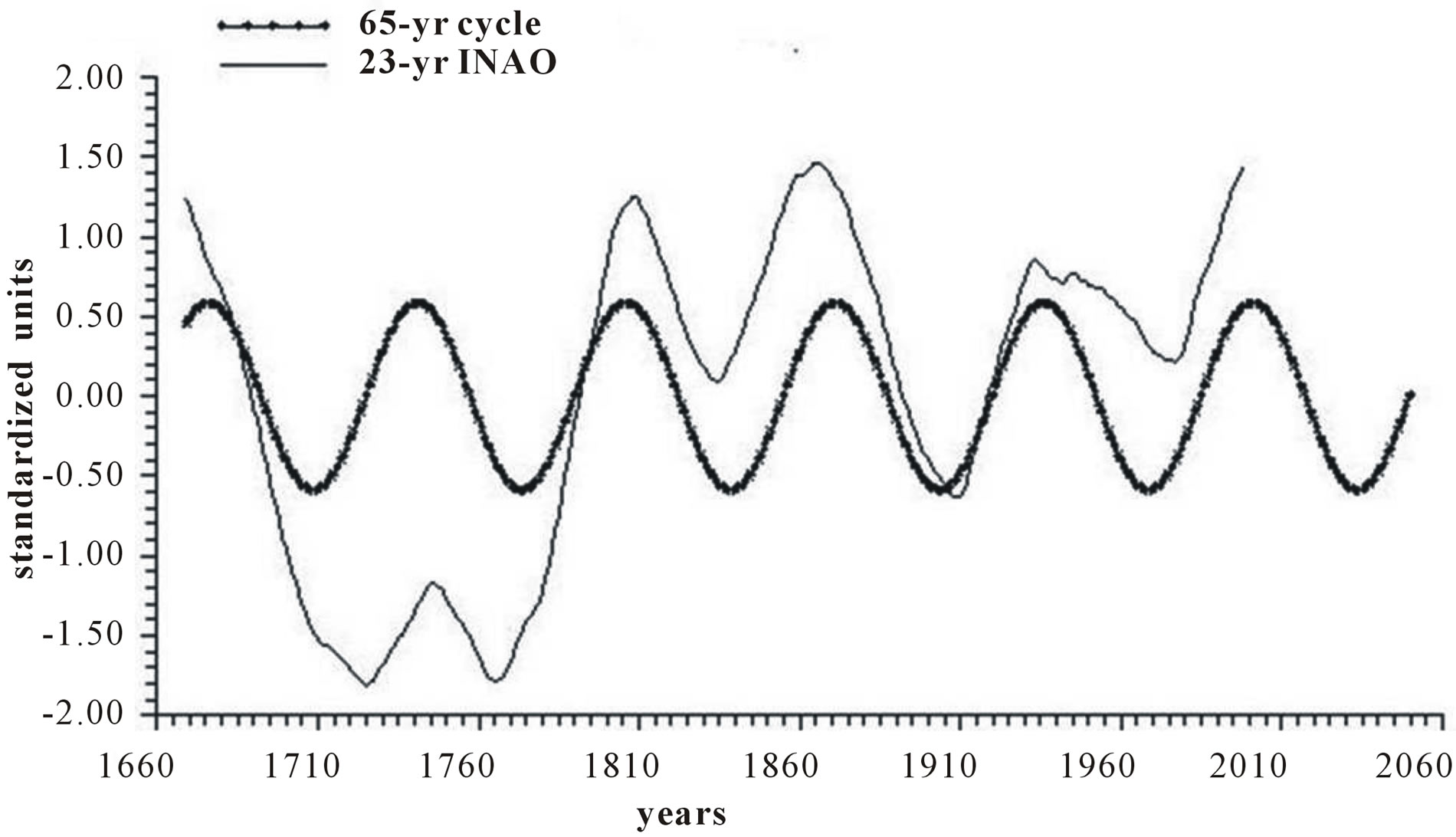
Figure 5. Time plot of yearly values of 23-yr INAO and of its 65-yr harmonic extrapolated in advance until 2060.
5. DISCUSSION
Length of day (LOD) is a good proxy for climatic changes under the assumption that it is the integral of the different circulations that occur within the ocean-atmosphere system both along latitude (zonal circulation) and longitude (meridional circulation) [4-6]. Here we have confined our investigation to NAO that is the main synodic mode of Northern hemisphere atmospheric circulation. For proper comparison between NAO and LOD climatic forecasting ability, we previously time-integrate NAO yearly values to obtain INAO yearly values that represent the Northern hemisphere zonal wind speed. In this respect, the 1785-1875 interval appears to have experienced strong zonal circulation while the 1700-1775 interval is characterized by weak zonal circulation (Figure 2). It is herein confirmed that LOD is inversely related to SST with a peak relationship when LOD is shifted ahead by 4 years and with a correlation coefficient gradually increasing from −0.66 to −0.79, to −0.89 and to −0.96 when moving from yearly values to those filtered with a moving average of order 5, 11 and 23 (Figure 3). INAO is found to be directly related to SST with a peak relationship when INAO is shifted ahead by 4 years and with a correlation coefficient gradually increasing from 0.74, to 0.89, to 0.95 and to 0.96 as we move from raw yearly values to values filtered with a moving average of order 5, 11 and 23. This indicates that an increase in zonal wind speed is responsible for an increase in SST in an ever more efficient way as the time scale of the averaging process increases (Figure 4). There is almost an equilibrium between zonal and meridional circulation: strong zonal circulations cause the contraction of the circumpolar vortex and an increase in air temperature while weak zonal circulations or, equivalently, strong meridional circulations with meandering or cellular patterns cause an expansion of the circumpolar vortex and a decrease in air temperature. Zonal epochs correspond to periods of global warming and meridional ones to periods of global cooling [4-6,17,18]. INAO values are found to be inversely related to those of LOD such that periods of increasing zonal wind speed are accompanied by periods of Planet increasing rotational rate while periods of decreasing zonal wind speed are accompanied by periods of Planet decreasing rotational rate [18]. On the other hand, the Medieval Warm Period known also as Medieval Climate Optimum was caused by a persistent and large positive NAO [19] that corresponds to high values of INAO. The correlation coefficients between INAO and SST are systematically higher on the various examined time scales in respect to correlation coefficients between LOD and SST and such results show that the INAO data are a more efficient proxy for climatic changes than LOD. The physical cause of the identified 65-year harmonic in INAO might be of astronomical type: the two giant planets, Jupiter and Saturn, have a period around the sun of 12 and 30 years, respectively and their least common multiple is equal to about 60 years, i.e., Earth, Jupiter and Saturn reach the same relative alignment around the sun after almost 60-yr [1,20].
6. CONCLUSION
The main physical and chemical processes inside the atmosphere-ocean system are governed by innumerable dynamic and thermodynamic parameters interconnected non-linearly, with an infinite degrees of freedom and currently unknown triggering processes. Such a complexity makes it difficult to adopt a strictly reductionist like GCM models and favours a holistic approach working outside the system. This drastically reduces the degrees of freedom on which the system operates and provides simpler and more reliable forecasting similar to those obtained in celestial mechanics in which the operative forces are described by a small number of equations. Here we have demonstrated a viable alternative to normal practice for forecasting climatic changes starting from not from GCM models but from INAO series. If INAO behaves in the same way in the future as in the past, the extrapolation of its dominant 65-yr harmonic might suggest a forecast estimate for a decline in SST starting from 2005, a result supported by recent data.
REFERENCES
- Mazzarella, A. and Scafetta, N. (2012) Evidences for a quasi 60-year North Atlantic Oscillation since 1700 and its meaning for global climatic change. Theoretical and Applied Climatology, 107, 599-609. doi:10.1007/s00704-011-0499-4
- Mc Lean, R.C. and Ivimey-Cook, W.R. (1973) Textbook of theoretical botany. Addison-Wesley Educational Publishers Inc., Upper Saddle River.
- Curry, J.A. and Webster, P.J. (2011) Climate science and the uncertainty monster. Bulletin of the American Meteorological Society, 92, 1667-1682. doi:10.1175/2011BAMS3139.1
- Mazzarella, A. (2007) The 60-year modulation of global air temperature: The Earth’s rotation and atmospheric circulation connection. Theoretical and Applied Climatology, 88,193-199. doi:10.1007/s00704-005-0219-z
- Mazzarella, A. (2008) Solar forcing of changes in atmospheric circulation, Earth’s rotation and climate. The Open Atmospheric Science Journal, 2, 181-184. doi:10.2174/1874282300802010181
- Mazzarella, A. (2009) Sun climate linkage now confirmed. Energy & Environmental Science, 20,123-130. doi:10.1260/095830509787689150
- Rogers, J.C. (1984) The association between the North Atlantic Oscillation and the Southern Oscillation in the northern hemisphere. Monthly Weather Review, 112, 1999-2015. doi:10.1175/1520-0493(1984)112<1999:TABTNA>2.0.CO;2
- Hurrell, J.W. (1995) Decadal trends in the North Atlantic Oscillation regional temperatures and precipitation. Science, 269, 676-679. doi:10.1126/science.269.5224.676
- Jones, P.D., Jónsson, T. and Wheeler, D. (1997) Extension to the North Atlantic Oscillation using early instrumental pressure observations from Gibraltar and South-West Iceland. International Journal of Climatology, 17, 1433- 1450. doi:10.1002/(SICI)1097-0088(19971115)17:13<1433::AID-JOC203>3.0.CO;2-P
- Luterbacher, J., Xoplaki, E., Dietrich, D., Jones, P.D., Davies, T.D., Portis, D., Gonzalez-Rouco, J.F., von Storch, H., Gyalistras, D., Casty, C. and Wanner, H. (2002) Extending North Atlantic Oscillation reconstructions back to 1500. Atmospheric Science Letters, 2, 114-124. doi:10.1006/asle.2001.0044
- Stephenson, F.R. and Morrison, L.V. (1995) Long-term fluctuations in Earth’s rotation: 700 BC to AD 1990. Philosophical Transactions A, 351, 165-202. doi:10.1098/rsta.1995.0028
- Brohan, P., Kennedy, J.J., Harris, I., Tett, S.F.B. and Jones, P.D. (2006) Uncertainty estimates in regional and global observed temperature changes: A new dataset from 1850. Journal of Geophysical Research, 111, D12106. doi:10.1029/2005JD006548
- Rayner, N.A., Parker, D.E., Horton, E.B., Folland, C.K., Alexander, L.V., Rowell, D.P., Kent E.C. and Kaplan, A. (2003) Globally complete analyses of sea surface temperature, sea ice and night marine air temperature, 1871- 2000. Journal of Geophysical Research, 108, 4407. doi:10.1029/2002JD002670
- Rossby, C.G. (1941) The scientific basis of modern meteorology in climate and man, in yearbook. US Department of Agriculture, Washington DC.
- Bath, A. (1974) Spectral analysis in geophysics. Elsevier, New York.
- Cecere, A., Mazzarella, A. and Palumbo, A. (1981) TIDE: A computer program of refinement of the ChapmanMiller method for the determination of lunar tides. Computers & Geosciences, 7, 185-198. doi:10.1016/0098-3004(81)90029-7
- Lamb, H.H. (1972) Climate, present, past and future. Methuen, London.
- Lambeck, K. (1980) The Earth’s variable rotation. Cambridge University Press, Cambridge. doi:10.1017/CBO9780511569579
- Trouet, V., Esper, J., Graham, N.E., Baker, A., Scourse, J.D. and Frank, D.C. (2009) Persistent positive North Atlantic Oscillation mode dominated the medieval climate anomaly. Science, 324, 78-80. doi:10.1126/science.1166349
- Scafetta, N. (2010) Empirical evidence for a celestial origin of the climate oscillations and its implications. Journal of Atmospheric and Solar-Terrestrial Physics, 72, 951-970.