Natural Science
Vol.5 No.1(2013), Article ID:26619,5 pages DOI:10.4236/ns.2013.51008
Nearest neighbor vector analysis of SDSS DR5 galaxy distribution
![]()
1American Physical Society, Maryland, USA; *Corresponding Author: yongfeng.wu@maine.edu
2Department of Astronautics Engineering, Harbin Institute of Technology, Harbin, China
3Department of Physics, University of Maine, Orono, USA
4Department of Mathematics, University of Maine, Orono, USA
Received 25 October 2012; revised 28 November 2012; accepted 10 December 2012
Keywords: Nearest Neighbor Distance; Nearest Neighbor Vector; Anisotropy; SDSS DR5; Galaxy Distribution
ABSTRACT
We present the nearest neighbor distance (NND) analysis of SDSS DR5 galaxies. We give NND results for observed, mock and random sample, and discuss the differences. We find the observed sample gives us a significantly stronger aggregation characteristic than the random samples. Moreover, we investigate the direction of NND and find the direction has close relation with the size of the NND for the observed sample.
1. INTRODUCTION
By the end of the 30s of last century, from the analysis of the position of galaxies on photographic film, Reference [1] found that the distribution of galaxies is not random and they aggregate obviously. Reference [2] statistically built simple galaxy clusters model with random distributions, but mismatched with the observation significantly. In the 50s, people [3,4] observed thousands of clusters, many constituted by large numbers of galaxies. Even when the galaxies seemed isolated, they still have kind of correlation and can be described by correlation function, power spectrum, and other mathematical tools. The use of correlation functions to describe galaxy clustering has become widespread in recent years [5,6]. The nearest neighbor [7,8] distance is an especially powerful tool to describe small scales structures, because it depends on all the moments of the correlation function [9], thus it is extremely useful for revealing some aspects hidden in the correlation functions [7]. Even if it only provides information of the clusters pattern within a rather restricted range of scales [10], interesting results were obtained when this method was applied to galaxy data and also mock galaxy catalogs draw from N-body simulations [11].
Compared to previous research, a significant difference of this paper is to develop the application of the Nearest Neighbor Vector (NNV) direction. Reference [12] mentioned that the angle of the two nearest neighbors of each galaxy can be used to discover the filaments. Here we regard the displacement between a galaxy and its nearest neighbor as a vector and discuss the direction distribution in the whole sphere. The motivation of this article is try to answer this question: is the universe clustered (by NND analysis)? If so, do galaxies have directional preference to select the nearest neighbor? By the size and direction analysis of the nearest neighbor, we could get more recognition about the hierarchical universe.
Our article is organized as follows: In Section 2 we present the nearest neighbor statistical scheme. In Section 3 we study the data from the SDSS DR5. We summarize the results in Section 4 and have conclusions in Section 5.
2. NEAREST NEIGHBOR VECTOR ANALYSIS
Reference [13] proposed the concept of the distance field. Suppose a given galaxy is in a three-dimensional coordinate system with Cartesian coordinates x, y, z. Let j be any other SDSS galaxy with Cartesian coordinates xj, yj, zj. For each galaxy the distance to its nearest neighboring object ri is computed as [14]
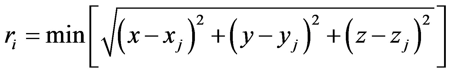 (1)
(1)
In this paper we simply use
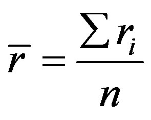 (2)
(2)
to calculate the average NND (nearest neighbor distance) in each sample. ri is the NND for each point and n is the total number of particles. According to [15], the random sample should have a value  equal to
 , the ratio
  could be used to measure the deviation from the random sample. For a random sample R = 1, for an extreme aggregation distribution (all points together), R = 0.
We also consider the direction of each NND in the distance field; we call it NNV (nearest neighbor vectors). We first construct a sphere to include all samples and then split the whole sphere into 180 triangles and investigate the distribution of NNV passing through each triangle. By analyzing the anisotropy of the NNV, we can find the footprint of the filaments and compare different samples in this way. The detailed description is in Section 4.
3. DATA
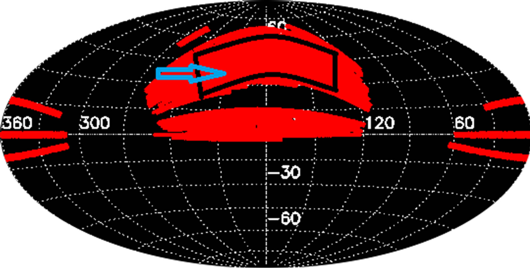
The Sloan Digital Sky Survey (SDSS) is one of the most ambitious and influential surveys in the history of astronomy. It is a major multi-filter imaging and spectroscopic redshift survey using a dedicated 2.5-m wideangle optical telescope at Apache Point Observatory in New Mexico, United States. We use the SDSS Data Release 5 as our galaxy sample, the detailed information (include the Redshift-distance formula, and a mock sample from Millennium Run Semianalytic Galaxy Catalogue [16] can be found from the paper of [17,18]. About 35,700 galaxies have been used after applying volumelimiting selection (e.g., [19]), which will ensure the selected galaxy sample is substantially complete to our absolute magnitude limit M = −19.9. See Figure 1 for the geometry of the sample.
4. RESULTS
For the observed sample we get 1.95 Mpc for average nearest neighbor distance, for the mock sample, we get 2.3 Mpc, and for the random sample we get rE = 3.5 ± 0.005 Mpc (11 random samples with different seeds). Then we have
 (3)
(3)
Clearly we can see observed sample has pronounced clustering on small scales compared with the random sample. Considering the extreme aggregation condition will have R = 0 and random sample has an R = 1, this observed sample is almost midway toward extreme aggregation. The clustering property of SDSS galaxies has been verified from various methods, such as two point correlation function [20-22]. The correlation length is about 5 - 7 Mpc [22] for Quasar and Luminous Red Galaxies (QSO-LRG). Our results of the average NND focus on more kinds of galaxies than QSO-LRG and support
 (a)
(a)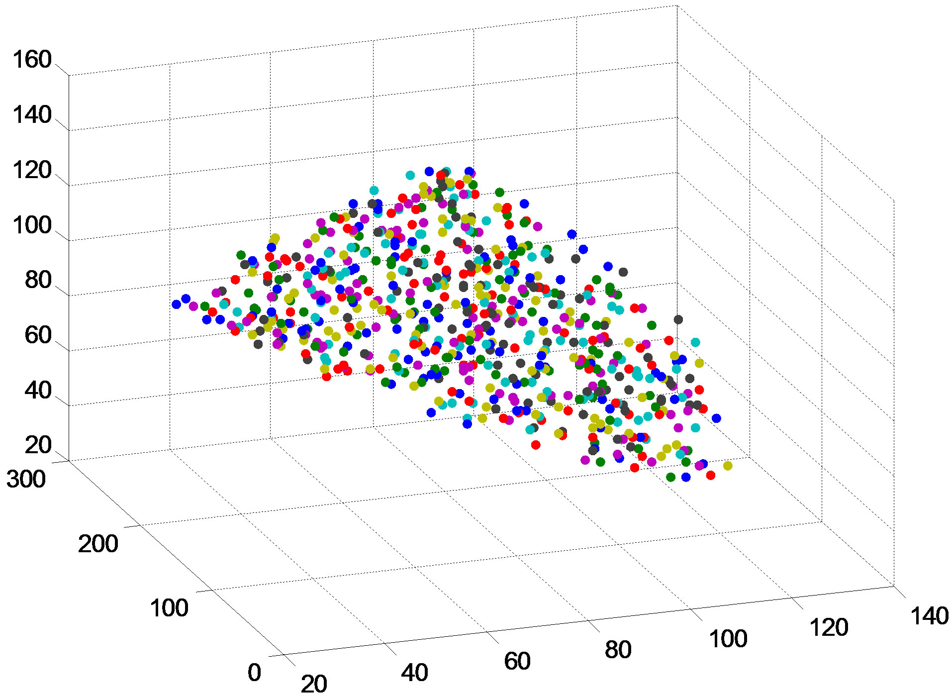 (b)
(b)
Figure 1. (a) SDSS sample geometry. The region inside the black “rectangle” of the figure is what we used; (b) 3D galaxy distribution, randomly (keep the original shape) selected hundreds galaxies from the observed sample.
this clustering property on small scale from a new way. The mock sample has a R = 0.66 in this measure value and is thus close to the observed sample.
Interestingly our analysis of the direction of the NND for each galaxy shows that the observed sample has an anisotropy property. To investigate the directional property of the NNV, we assumed all directions begin from a single point at origin, we split the whole surface of a sphere around the origin into 180 triangles (we could use the healpix method [23] to partition the surface into equal area “pixels”, but the pixels are different triangular shape) displayed from the top to the bottom in the sequence, see Figure 2.
In Figure 2(a) we have 120 triangles belonging to the hexagons and 60 triangles belonging to the pentagons. They (such as triangle 2 and triangle 7) do not have the same area size as they belong to two different kinds of polygons, pentagon and hexagon. So we put a weight 1.26 on pentagon triangles to compensate for the smaller area comparable to the hexagon triangles, so the total number of NNV on all triangles will be around 8% larger than the total galaxies. If we plot all NNV of galaxies together (put the origin point at (0, 0, 0)), we can get a sketch of directions like Figure 2(b).
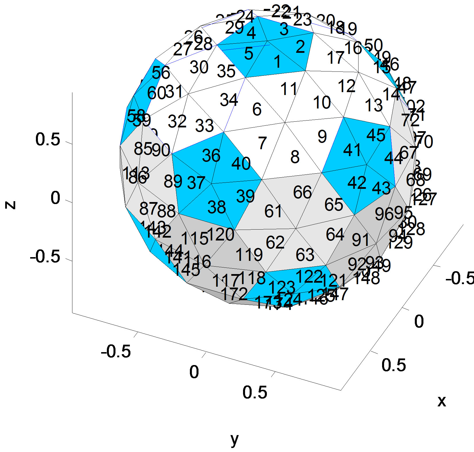 (a)
(a)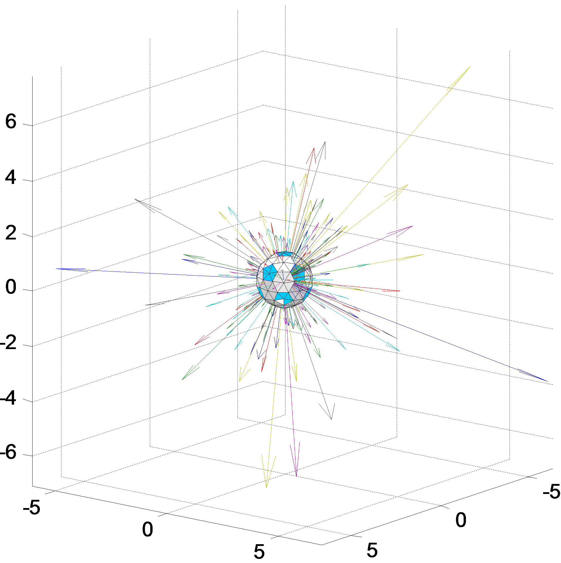 (b)
(b)
Figure 2. (a) The triangle surface of the sphere, the blue parts are pentagons and the white parts are hexagons; (b) An example of a NNV figure, each arrow represents the direction of the nearest neighbor of each galaxy and the length of the arrow represents the value of the NND, here we only plot 270 NNVs.
We collect the NNV for all galaxies first, and then as we know the 3-D coordinates of the three vertexes of the each triangle and the direction of NNV, we could precisely calculate which nearest neighbor vector crosses and plot them with the sequence of 180 triangles and get the distribution in Figure 3.
We also compute 11 random samples with different seeds to estimate the deviation. For all angles, mean value is 210 and we find that the average standard deviation (σ) is around 14 (maximum is 20) for all angles, in the following places all σ are taken from here.
Here some peaks are separated only because the arrangement of 180 triangles is arbitrary, so even two adjacent triangles may have dozens of serial number difference. Observed sample and mock sample looks very different at some specific triangles, but this is normal as the N-body simulation only simulate universe statistically, not exactly same with all details, such as the orientation of filaments. So we only focus on the global statistical properties from Figure 3(a), not specific angles.
From Figure 1, our sample geometry looks like a distorted solid angle; how does this affect the NNV analysis? Figure 3 clearly tells us we do not need to worry about it as random samples have almost same distribution on all 180 triangles with the same geometry of observe and mock sample.
In Figure 3 we clearly see observed sample has a strong NNV distribution on some triangles, which are around triangle 20, 50 and corresponding opposite direction triangle 140 and 170 (for pairs of galaxies, two NNV directions are opposite). To investigate the relation between NNV and NND, we split galaxies into two groups, one has a smaller NND than average, and another has a
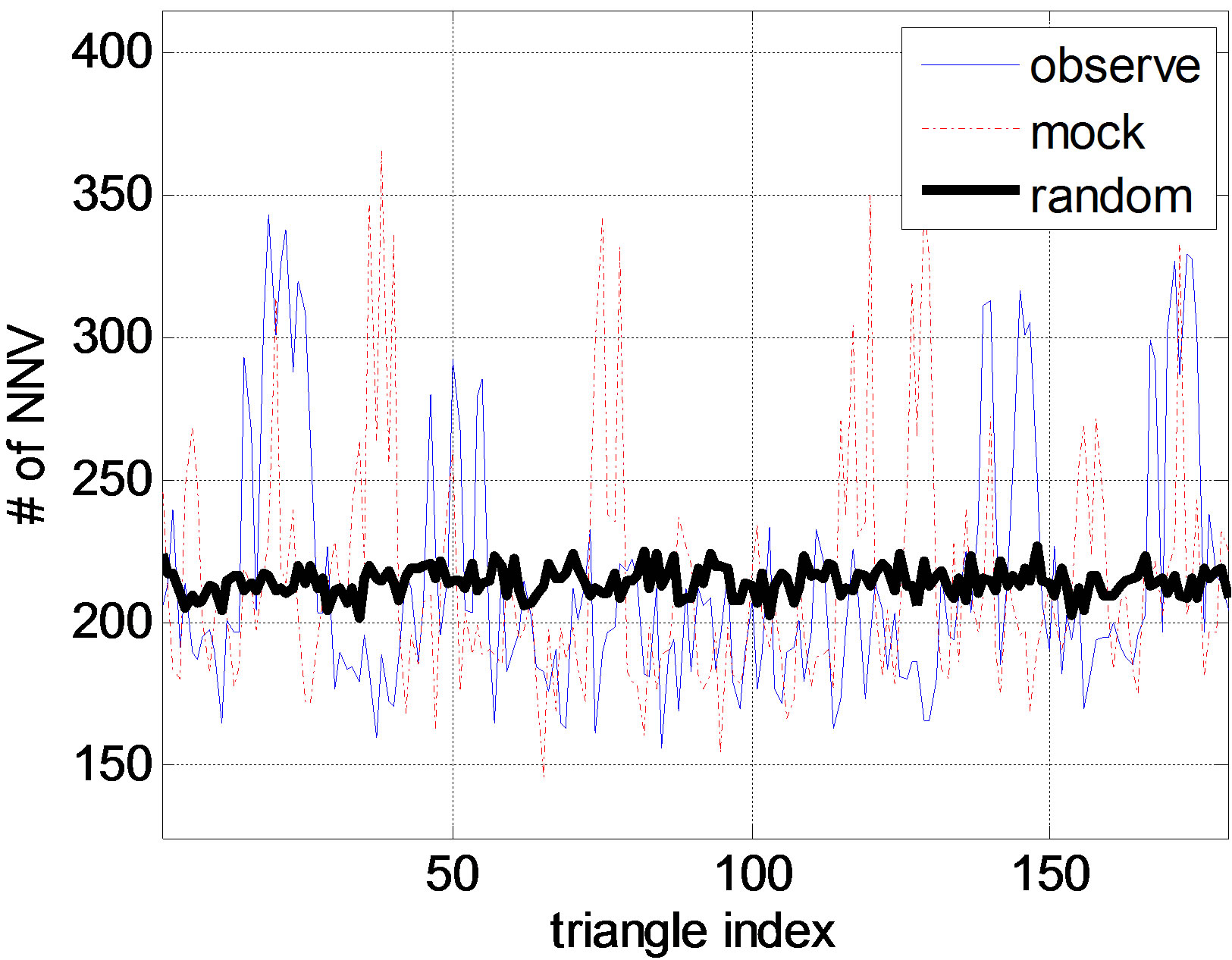 (a)
(a)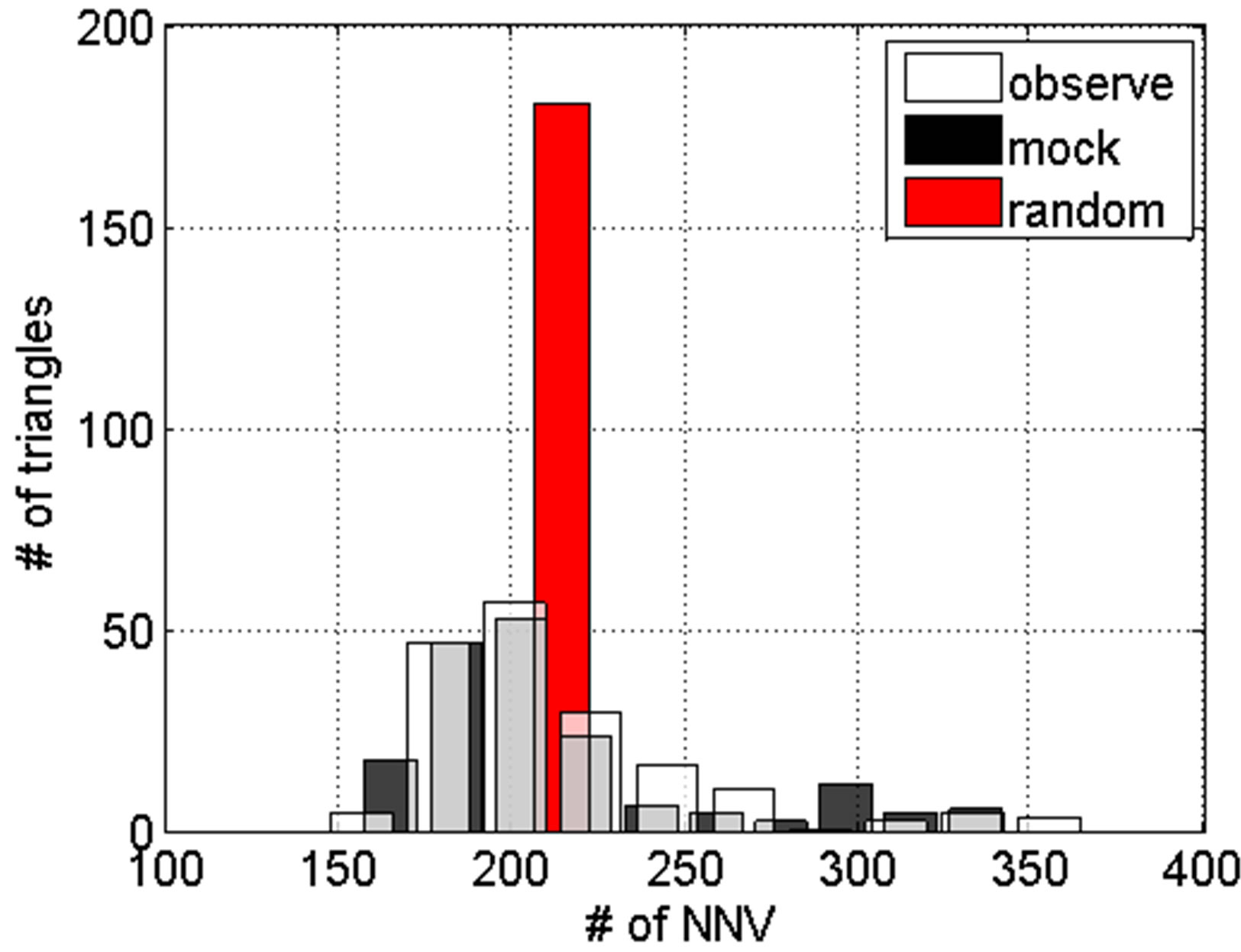 (b)
(b)
Figure 3. (a) NNV distributions on 180 angles for observe, mock, random samples; (b) Corresponding histogram for 3 samples. Overlap areas have gray color.
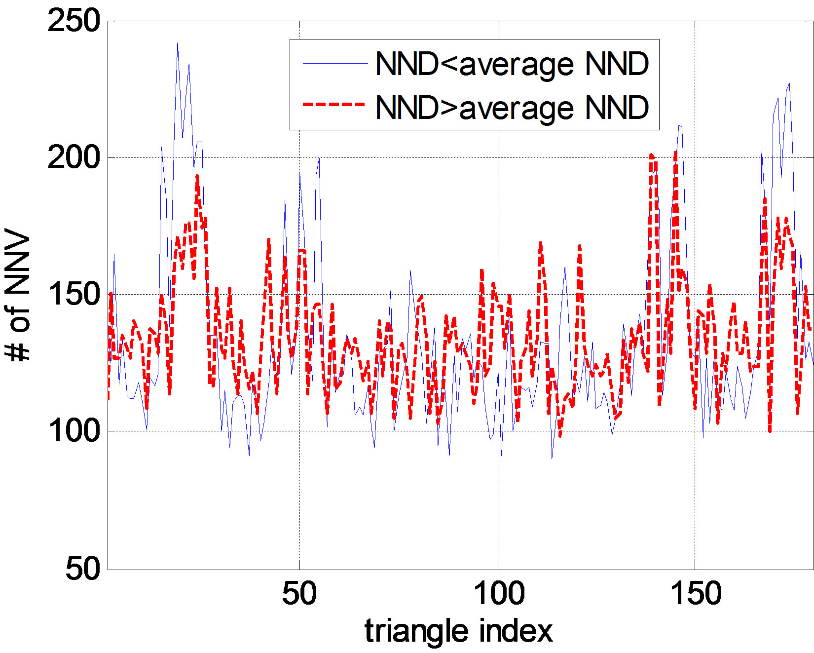
larger NND than average. We plot them in Figure 4 (two groups are normalized to have the same total number of NNVs).
We can see for smaller NND less than average, it displays a stronger anisotropy than galaxies have larger NND than average from Figures 4(a) and (b).
5. CONCLUSIONS
We have calculated the average NND of the SDSS galaxy sample and mock samples. We find the observed sample has a lightly smaller NND than mock sample, but much smaller than random sample. This result indicates observed sample is more clustered in a special way. Moreover, we use a new method to investigate the direction distribution of NNV and find the NNV of observed sample has a global anisotropy and is similar with mock sample, but clearly different from random sample on some angles. Figure 3(b) shows the distribution of the random sample is like a delta function and this reflects the expected isotropic distribution. The result from the
 (a)
(a) (b)
(b)
Figure 4. (a) NNV distribution for two kinds of galaxies: one kind has NND < 1.95 (average NND), another has NND >1.95; (b) Corresponding histogram for 2 kinds of sample.
observed sample is more like a Poisson distribution and this leads us think about the Gaussian fluctuations of cosmic microwave background (CMB). Both of them show the anisotropy resulting from the evolution of the universe, but with somewhat different statistical property. Maybe it is because our sample size is limited and needs further observations.
As both NNV and NND display significant difference between observed and random sample, this makes us think whether the NNV and NND are correlated. Figures 4(a) and (b) show that galaxies with smaller NND have stronger antistrophic NNV.
To better understand the physical sense of the results above, we shall check on the hypothesis about a global isotropic universe. There is a distinct hierarchy on a larger scale from a few hundred kpc to a few hundred Mpc [24]. Galaxies build up groups, clusters and superclusters, which in turn form a cellular structure of the Universe. We would expect the observed sample has strong clustering property and a smaller NND than random sample; this is coincident with the NND results we find. However, the results of NNV reflect the anisotropy of a hierarchical universe in a very way more than the cluster property. Even in a much clustered point distribution, we still could get an isotropic NNV distribution, say, some symmetric spherical galaxy clusters, or some thin filaments (assume the thickness only includes one galaxy) uniformly distributed on all directions. So the NNV analysis provides a new way to distinguish how hierarchy is organized for the universe and we find galaxies do have a directional preference to select the nearest neighbor in universe.
6. ACKNOWLEDGEMENTS
The project is supported by key laboratory opening funding of the Harbin Institute of Technology (HIT.KLOF. 2012.077).
REFERENCES
- Hubble, E.P. (1937) The observational approach to cosmology. The Clarendon Press, Oxford.
- Neyman, J., Scott, E.L. and Shane, C.D. (1953) On the spatial distribution of galaxies: A specific model. Astrophysical Journal, 117, 92. doi:10.1086/145671
- Abell, G.O. (1958) The distribution of rich clusters of galaxies. A catalogue of 2712 rich clusters found on the National Geographic Society Palomar Observatory Sky Survey. Astrophysical Journal, 3, 211.
- Zwicky, F., Karpowicz, M., Kowal, C.T., Herzog, E. and Wild, P. (1961) Catalog of galaxies and of clusters of galaxies (CGCG) Calif. Institute of Technology, Pasadena, 196.
- Peebles, P.J.E. (1973) Statistical analysis of catalogs of extragalactic objects. I. Theory. Astrophysical Journal, 185, 413-440.
- Cao, L., Liu, J.R. and Fang, L.Z. (2007) Estimating power spectrum of Sunyaev-Zeldovich effect from the cross-correlation between the wilkinson microwave anistropy probe and the two micron all sky survey. Astrophysical Journal, 661, 641-649. doi:10.1086/516775
- Ripley, B.D. (1981) Spatial statistics. Wiley, New York. doi:10.1002/0471725218
- Baddeley, A.J., Kerscher, M., Schladitz, K. and Scott, B. (2000) Estimating the J function without edge correction. Statistica Neerlandica, 54, 1-14. doi:10.1111/1467-9574.00143
- Bahcall, J. and Soneira R.M. (1981) The distribution of stars to V = 16th magnitude near the north galactic pole— Normalization, clustering properties, and counts in various bands. Astrophysical Journal, 246, 122-135. doi:10.1086/158905
- Cressie, N. (1991) Statistics for spatial data. John Wiley & Sons, New York.
- Kerscher, M., et al. (1999) A global descriptor of spatial pattern interaction in the galaxy distribution. Astrophysical Journal, 513, 543-548. doi:10.1086/306902
- Batuski, D.J. and Burns, J.O. (1985) A possible 300 megaparsec filament of clusters of galaxies in PerseusPegasus. Astrophysical Journal, 299, 5-14.
- Stavrev, K.Y. (1990) Large voids of rich clusters of galaxies. Eötvös University, Eötvös, 115.
- Allam, S.S. (2005) A catalog of very isolated galaxies from the sloan digital sky survey data release 1. The Astronomical Journal, 129, 2062-2073. doi:10.1086/428754.
- Clark, P.J. and Evans, F.J. (1954) Distance to nearest neighbor as a measure of spatial relationships in populations. Ecology, 35, 445-453. doi:10.2307/1931034
- Croton, D.J., et al. (2006) The many lives of active galactic nuclei: Cooling flows, black holes and the luminosities and colours of galaxies. Monthly Notices of the Royal Astronomical Society, 365, 11-28. doi:10.1111/j.1365-2966.2005.09675.x
- Wu, Y., Batuski, D.J. and Khalil. A. (2009) Multi-scale morphological analysis of SDSS DR5 survey—Using the metric space technique. Astrophysical Journal, 707, 1160- 1167. doi:10.1088/0004-637X/707/2/1160
- Wu, Y., Batuski, D.J. and Khalil. A. (2012) Three dimensional filamentation analysis of SDSS DR5 Survey. ISRN Astronomy, 2012, Article ID: 171829.
- Davis, M. and Peebles, P.J.E. (1983) A survey of galaxy redshifts. V. The two-point position and velocity correlations. Astrophysical Journal, 267, 465-482. doi:10.1086/160884
- Vasilyev, N.L. (2008) Correlation analysis of large-scale structure using data from the SDSS DR5 LRG catalog. Astrophysics, 51, 320-335.
- Ross, N.P., et al. (2009) Clustering of low-redshift (z ≤ 2.2) quasars from the Sloan Digital Sky Survey. Astrophysical Journal, 697, 1634.
- Mountrichas, G., et al. (2009) QSO-LRG two-point crosscorrelation function and redshift-space distortions. Monthly Notices of the Royal Astronomical Society, Vol. 394, 2050-2064.
- Calabretta, M.R. and Roukema, B.F. (2007) Mapping on the HEALPix grid. Monthly Notices of the Royal Astronomical Society, 1-8.
- Weinberg, D.H. (2005) Mapping the large-scale structure of the universe. Science, 309, 564. doi:10.1126/science.1115128