Engineering
Vol. 4 No. 7 (2012) , Article ID: 20537 , 4 pages DOI:10.4236/eng.2012.47051
Optimality Conditions and Algorithms for Direct Optimizing the Partial Differential Equations
Computer Science Department, Donetsk National University, Donetsk, Ukraine
Email: tvk@dongu.donetsk.ua
Received April 20, 2012; revised May 17, 2012; accepted May 26, 2012
Keywords: Optimization; Gradient; Necessary Conditions for Optimality; Partial Differential Equations; Infinite-Dimensional Algorithms
ABSTRACT
New form of necessary conditions for optimality (NCO) is considered. They can be useful for design the direct infinitedimensional optimization algorithms for systems described by partial differential equations (PDE). Appropriate algorithms for unconstrained minimizing a functional are considered and tested. To construct the algorithms, new form of NCO is used. Such approach demonstrates fast uniform convergence at optimal solution in infinite-dimensional space.
1. Introduction
Three classes of optimization problems for PDE are known, e.g., [1]: optimal control, parameter identification, and optimal design. To solve its in general case are used optimization algorithms in infinite-dimensional spaces, and finite-dimensional spaces. In the last case the algorithms are applied after transformation a desired parameter-function into a finite-dimensional space. We shall consider direct optimization [2,3], i.e. immediately minimization an objective functional  by infinite-dimensional methods on the basis of the gradient
 . Here
  is a Frechet derivative, which is a linear functional. It depends on desirable parameter
  and space-time variable
 .
.
It is well known classical NCO for unconstrained optimization problems:
 (1)
(1)
where  is an optimum value of a desired parameter,
  is a space of desired parameters defined on
 ,
,  is an adjoint space.
Because of computing errors the NCO (1) is never implemented. Approximate value of (1) is used sometimes for estimating a relative minimization of  in linear search problems. Sometimes approximate value of (1) is used as a completion criterion for optimization. No one uses NCO (1) for choosing a minimization direction in optimization algorithms.
We will consider NCO in a new form. It can be used for choosing a minimization direction for direct optimization algorithms.
2. Necessary Condition and Optimization Algorithm
2.1. Algorithm
For direct minimization approach the solution  is searched on the basis of the algorithm
 (2)
(2)
where direction  is a linear functional representing the anti-gradient of the objective functional, here
 , or the conjugate gradientse.g. Polak-Ribière (CG-PR)
 ,
,  ,
,  is a step-size.
Unfortunately, the optimizing by the algorithm (2) is not always possible. Even for a quadratic J there are no grounds of convergence for infinite-dimensional algorithm (2).
Let’s replace (2) by the following algorithm:
 (3)
(3)
where  is a function which regulates a convergence
  on each iteration.
2.2. Necessary Condition
How correctly to set a function  in (3)? Let’s require: the algorithm (3) has to provide almost everywhere on
  (a.e.
(a.e. ) convergence in an adjoint space
 . Thus instead of integral NCO (1) we must to introduce the following NCO.
Theorem. Let  be a smooth unconstrained functional, and it has a strict minimum at
 . Then in some neighborhood of
  the sequence
  exists such, that
 a.e.
a.e. . (4)
. (4)
The singularity of introduced NCO (4) is that it is imposed on the gradient in vicinity of a minimum  instead of not exactly at
  as it is presented in (1). Therefore the condition (4) can be used for constructing minimization steps near
 . We are going to use new NCO (4) to set a function
  for algorithm (3).
The algorithm (3) with implementation of (4) allows us to solve infinite-dimensional optimization problems, under assumption that from a convergence a.e. in an adjoint space
  the similar convergence follows in a primal space
 .
.
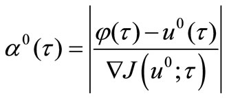
For a quantitative estimation of condition (4) let’s introduce NCO-function
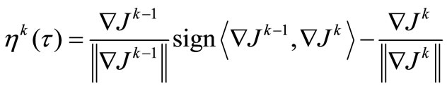 ,
,
For this function, it is possible to write the NCO (4) in a more strong form
 . (5)
. (5)
The NCO-Theorem with (5) instead of (4) requires decrease of function  not only a.e.
 , but proportionally a.e.
 for each iteration
  under driving to
 . The analogy in a finite-dimensional space for condition (5) denotes that the gradients vectors have to be collinear for all iterations up to
  [4].
[4].
2.3. Implementation
The difficulty of practical implementation of method (3) is contained in a selection of function  for satisfying the NCO (4) or (5). Consider one of methods for approximate implementing (5) on initial iterations.
We need to introduce a concept of template approximations. Let initial  and
and  known. Let’s set the first approximation
 , where
  is a template function, for which the gradient
  satisfies to (5), i.e. proportionally decreases after the first iteration. Thus from (3) we can find, under
 :
:
 ,
, .
.
On the following iterations we set parameter 
 . In the given method from the researcher it is required to make some first experimental iterations for selecting an appropriate template function
 , which satisfies to NCO (5).
We call your attention that the described method for  can be applied to such
 , that
 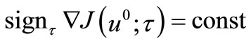 , i.e. when
 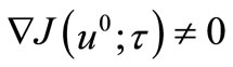 for all
 .
.
2.4. Example
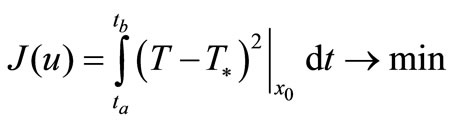
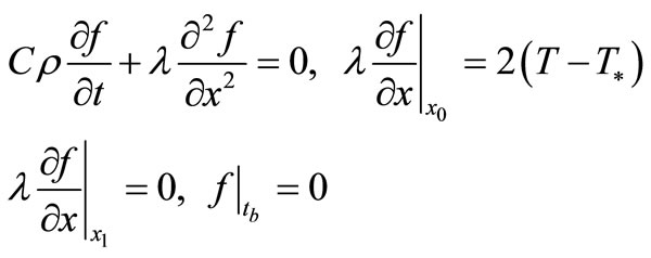
As an example we shall consider a one-dimensional linear parabolic heat equation in area
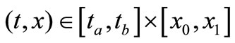 :
:
 (6)
(6)
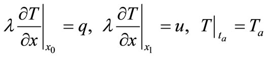
where  is a temperature,
  ,
,  , and
, and  is a thermal capacity, a density, and a thermal conduction accordingly. It is necessary to find a heat flow
  on bound
  (set
(set ) that keeps a temperature
  on other bound
  for given outflow
 :
:
 (7)
(7)
Applying the adjoint variables, we find the gradient
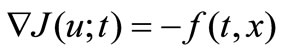 on
on where
where 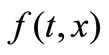 is a solution of the following adjoint problem
The curve 1 on Figure 1 illustrates unsuccessful attempt of solving the problem (6), (7) by infinite-dimensional algorithm (1) with direction  from method CGPR. At initial approximation
 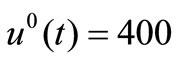 kJoule/(m2·s) and optimal
  kJoule/(m2·s) the gradient has very non-uniform value on segment
 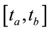 (up to 7 orders) and, as a corollary, we obtain a non-uniform convergence to
  by method CG-PR.
The attempt of solving the problem by finite-dimensional optimization algorithms has not given a positive outcome. Next we tried to do expansion of function  through B-splines of zero order (piece-wise functions) with carriers equal to time-step
  as it was made in [5]. Given this, the finite-dimensional control
 ,
,  , was found by quasi-Newton method BFGS [6,7]. The solution coincided with the previous curve 1 on Figure 1.
All minimizing was finished under relative change of  and
and  less than 1%. It is necessary to notice, that
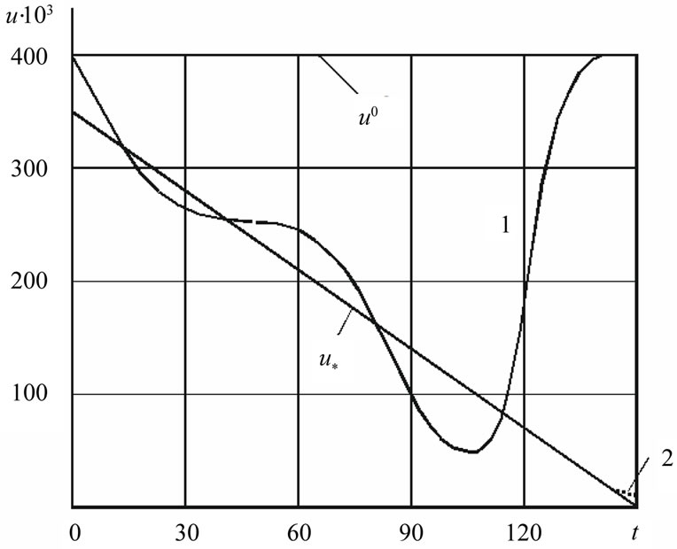
Figure 1. Solution of optimal control problem. 1: methods CG-PR and BFGS; 2: method (3); u0: initial approximation; u*: exact solution.
the further iterating for method BFGS has allowed it to minimize J better than CG-PR. However, the curve 1 has varied not in essence. The outcomes speak that the optimization even with linear systems, which governed by PDE, is not always possible by traditional infinite-dimensional and finite-dimensional methods.
The curve 2 on Figure 1 is a solution of problem (6), (7) by new infinite-dimensional method (3) under  chosen by method CG-PR with template function
 (8)
(8)
The given function satisfies the NCO (4). We tried the second template function as:
 (9)
(9)
It satisfies the strong NCO (5). Here solution has coincided with  precisely on Figure 1.
To select a function  we analyze a behavior of function
 . A value of this function for all methods on the first experimental step
  is shown in Figure 2. We see, that the classical methods CG-PR, BFGS (see the curve 1) realize the new NCO badly, to be exact, they do not implement its. Method (3) with
  in (8) (see the curve 2) not bad implements NCO (4), but does not implement strong NCO (5). Method (3) with
  in (9) (see the curve 3) implements strong NCO (5) and provides convergence to exact solution
  better all especially on the first iterations.
It is necessary to tell, that the template functions  in (8) and (9) give noticeably different minimization outcomes only on the first iteration. With growth of iterations they give approximately equal good outcomes. It is explained to that the parameters
 , regulating a descent in method (3), are computed with the account of NCO only on the first step. For discussed method
  .
.
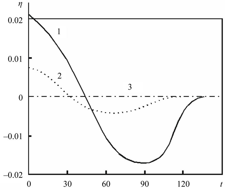
Figure 2. NCO-function η(t) for first experimental step. 1: method CG-PR; 2: method (3) with NCO (4); 3: method (3) with strong NCO (5).
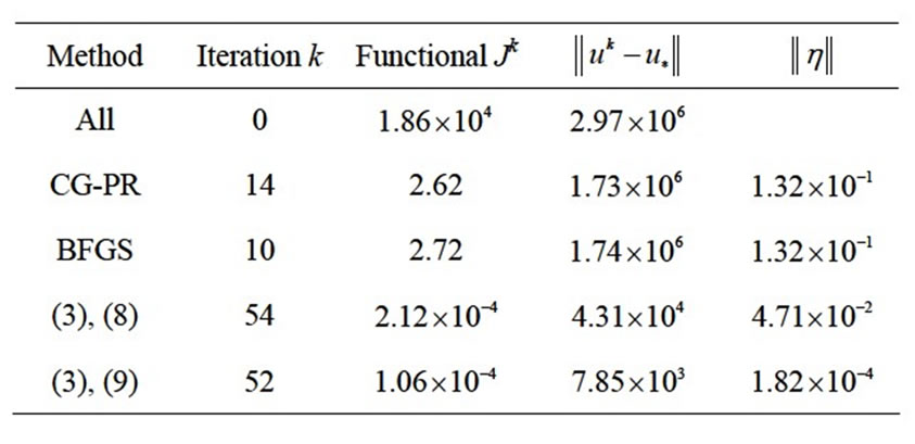
Table 1. Initial and final values of the objective functional, the proximity to an exact solution, and strict NCO (on a first experimental step).
Everywhere for searching a step-size , the method Wolfe with quadratic interpolation was used (Wright, Nocedal, 1999). Here step-size was computed from conditions
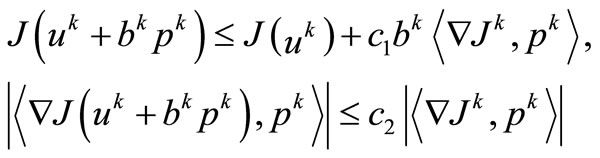 (10)
(10)
The parameters of a method were given  and
and .
.
In the Table 1 are shown the obtained values of the objective functional, the proximity to exact solution, and NCO (5) (on a first step) for all methods. From outcomes of computations it is seen, that the new method on the basis of algorithm (3) with NCO (5) minimizes the functional J on 4 orders better than the traditional methods. The method has allowed us to approach to optimal solution  on 3 orders closer.
3. Conclusion
Thus, the new NCO has appeared effective for constructing the algorithms of direct optimization for processes which governed by PDE. The algorithm (3) with NCO (4) or (5) can be recommended to solving the infinite-dimensional optimization problems.
REFERENCES
- N. M. Alexandrov, “Optimization of Engineering Systems Governed by Differential Equations,” SIAG/OPT Views & News, Vol. 11, No. 2, 2000, pp. 1-4.
- R. M. Lewis, “The Adjoint Approach in a Nutshell,” SIAG/OPT Views & News, Vol. 11, No. 2, 2000, pp. 9-12.
- V. K. Tolstykh, “Direct Extreme Approach for Optimization of Distributed Parameter Systems,” Yugo-Vostok, Donetsk, 1997.
- V. K. Tolstykh, “New First-Order Algorithms for Optimal Control under Large and Infinite-Dimensional Objective Functions New First-Order Algorithm for Optimal Control with High Dimensional Quadratic Objective,” Proceedings of the 16th IMACS World Congress on Scientific Computation, Applied Mathematics and Simulation, Lausanne, 21-25 August 2000. http://metronu.ulb.ac.be/imacs/lausanne/CP/215-3.pdf
- R. H. W. Hoppe and S. I. Petrova, “Applications of the Newton Interior-Point Method for Maxwell’s Equations,” Proceedings of the 16th IMACS World Congress on Scientific Computation, Applied Mathematics and Simulation, Lausanne, 21-25 August 2000. http://metronu.ulb.ac.be/imacs/lausanne/SP/107-7.pdf
- C. T. Kelly, “Iterative Methods for Optimization,” SIAM, Philadelphia, 1999. doi:10.1137/1.9781611970920
- J. Nocedal and S. J. Wright, “Numerical Optimization,” Springer, New York, 1999. doi:10.1007/b98874