Journal of Modern Physics
Vol.3 No.9(2012), Article ID:22647,4 pages DOI:10.4236/jmp.2012.39123
Line Shapes in the Magnetized Plasmas
1Lycée Professionnel Léonard de Vinci, Marseille, France
2Department of Physics, Laboratory of Research in Plasma and Surface, University of Ouargla, Ouargla, Algeria
Email: *ktouati@yahoo.com
Received July 11, 2012; revised August 22, 2012; accepted August 29, 2012
Keywords: Line Profiles; Radiation Polarization; Stark Effect; Zeeman Effect
ABSTRACT
Till now, the most studies of Lyman alpha line are concerned only by the Stark effect. In our knowledge few investigations are developed for the plasmas subjected to a magnetic field. In this paper we present the combined effect, StarkZeeman, on the spectral line shape. The dynamic effects due to the time fluctuation of the electric microfield and the radiation polarization are also taken into account.
1. Introduction
In plasmas, the emitter atoms can be well represented by the spectral line shapes. These are, combined with an adequate theory, important tools of diagnostic of densities and temperatures in astrophysical and laboratory plasmas as in the fusion experiences. Most of the works on Lyman alpha lines, up to new, are only concerned the Stark effect whereas a very little investigation has been done on the plasmas in the presence of an external magnetic field (combined Stark-Zeeman effects). We observe today a lot of plasmas where magnetic fields reign: Astrophysics (magnetic stars, white dwarf, neutron stars), high density energy plasma and magnetic fusion (tokamaks, stellator, pinch). To shake off the difficulties related to the complexity of different mechanisms of the broadening, the theory must consider nearly the interaction between the emitter and all the plasma in one part and between the emitter and the external fields, electric and magnetic, in other part, without neglecting the internal structure of the emitter. In this work, we have presented a model of the absorption or emission lines that relay on the distinction between the emitter atom as a quantal system with a high number of levels and its environment in presence of a constant external magnetic field. In presence of magnetic field, the emitted light is polarized. In this case, the line shape depends on the observation direction and also on the electric field direction with respect to the external magnetic field direction. This dependency makes the calculations very difficult because, in the presence of an external magnetic field, the hypothesis of the isotropic plasma is not valid. We have then thought to fix the direction of observation and to consider all the possible directions of the ionic microfield E. We have then developed in this work the general theory of the broadening of the spectral line shape in the magnetized plasmas using the framework of the time dependent perturbations theory.
2. Transitions Probabilities
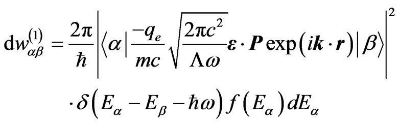
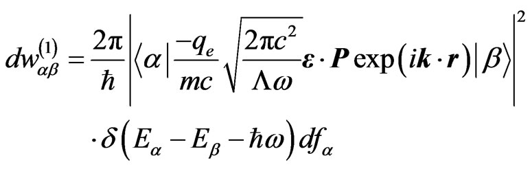
We use the time dependent perturbations theory to describe the transitions probabilities between the states α and β which are given by [1]:
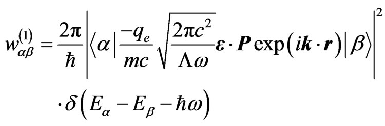 (1)
(1)
where m and r are the electron mass and the position operator respectively, whereas P and  are the polarization vector and its unit vector of the photon.
The radiation is specified by the frequency  and the wavelength vector
 .
.  is the volume of the radiative system and c is the light velocity. Let
  the number of states whose energy is in the infinitesimal band
 ;
; . The transition probability from the state
  to a state whose energy is in this band can be written as:
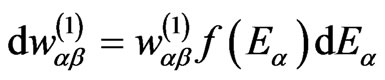 (2)
(2)
Inserting (1) in (2), we find:
 (3)
(3)
Or:
 (4)
(4)
Assuming that the polarization of the radiation is well determinated and the radiation propagating in the solid angle  and using [2]:
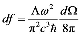 (5)
(5)
we find the absorption probability including one photon as:
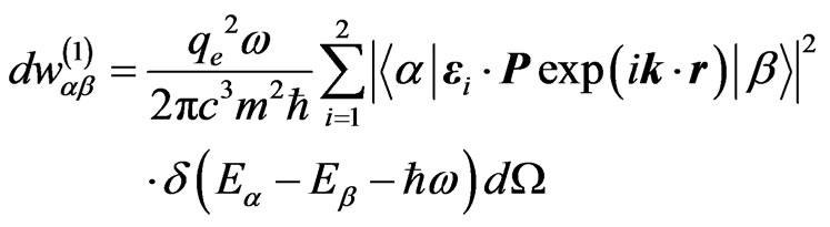 (6)
(6)
The last formula translates the probability that the bounded electron of the radiative system absorb in unit time one photon with energy , a wavelength k and a polarization
 . The sum concerns the possible two independent transversal polarizations. In the electric dipolar approximation, the last formula, multiplied by the photon energy
  and summed on all initial and final states concerned by the transition, gives the total emitted power as follows:
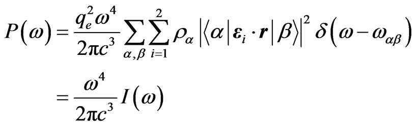 (7)
(7)
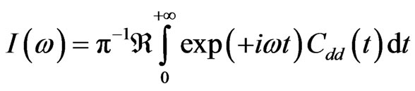
where  is the intensity of the spectral line.
3. The Spectral Line in Magnetic Field: The Line Stark-Zeeman
We shall restrict our studies by taking the non-quenching hypothesis and then we adopt the notation used by Baranger [2] for the “double-atom” for which the radiative transition are only allowed between the upper level  and lower level
  because
  and
and . The emitted light in the presence of the magnetic field or the electric field is polarized and then the line shape depends on the observation direction. This alternative yields the calculation very hard. One simplification consists to consider the space isotropy and then to take only one observation axis independently of the polarization. However this approach ceases to be valid when a magnetic field is present. It must then to fix an observation axis and to consider all the possible angles between the magnetic and ionic electric field. The spectral line turn out to depend on the observation axis in one part, and on the system geometry
  in other part.
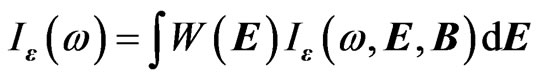
4. The Line Stark-Zeeman: Quasi-Static Approximation
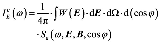
As seen the line shape  must includes all polarizations and the angles between the ionic electric field
  and the magnetic field
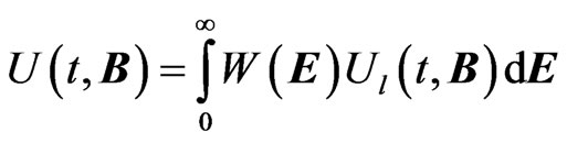
 . The use of the Fourier transform allows us to define a time-dependent function
 , a time-dependent auto-correlation function of the dipole momentum. The later can be written as [3]:
 (8)
(8)
and
 (9)
(9)
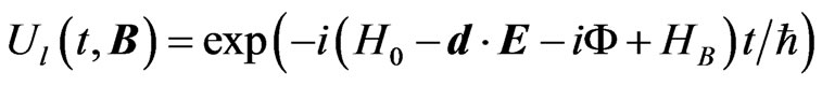
The evolution operator , for a constant ionic field
  is:
is:
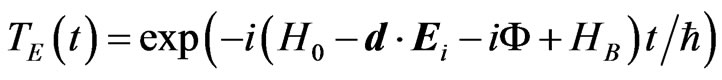 (10)
(10)
where  is Zeeman effect and
 . describes the electron collisions. The mean value of the evolution operator is obtained when we average on all possible configuration of the ionic field. This can be achieved by taking the distribution function of the field
 :
:
 (11)
(11)
For a given polarization direction, and if  is not perturbed by the presence of the magnetic field, the spectral line is written as:
 (12)
(12)
Note k be the observation direction, take two independent polarization directions  and
and  and assume in the subsequently that
  is oriented towards Oz axis. To take into account the effect of the direction of the ionic field
 , we must rotate it about the magnetic field
  for all angles. The independent polarizations
  and
and  are perpendicular and parallel respectively to the plane (P) lying to
  and
and . Let be
  the azimuthal angle between (P) and xOz plane whereas
  is the angle between
  and
and .
.
The polarizations ,
,  are defined in the frame O xyz (see Figure 1) as:
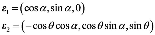 (13)
(13)
For each relative direction of  and
and  the spectral
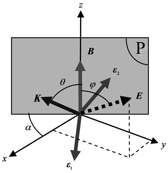
Figure 1. Geometry showing the polarizations and the magnetic field.
line is noted by 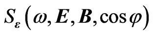 where
where  refers to the angle between
  and
and , then:
 (14)
(14)
Or:
 (15)
(15)
Projecting  on ox, oy, oz axis, we find for each direction of the polarizations
  and
and  [4]:
[4]:
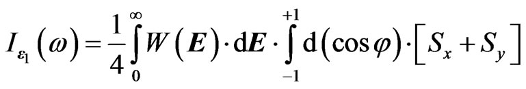 (16)
(16)
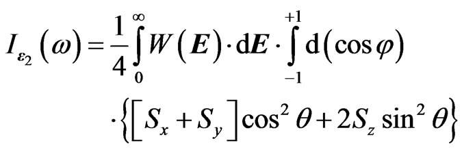 (17)
(17)
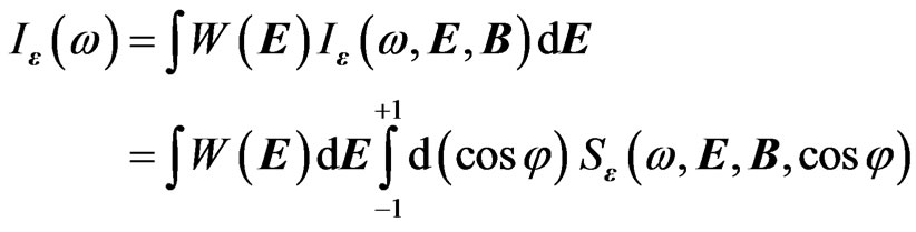
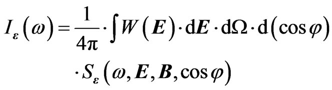
If we omit the distinction between the polarization directions, we find:
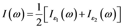 (18)
(18)
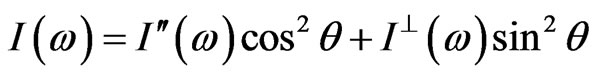
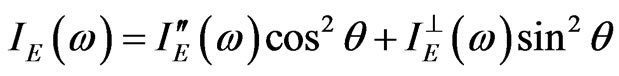
The longitudinal and the transversal observations with respect to the magnetic field direction allow us to define two intensities, say parallel and perpendicular as:
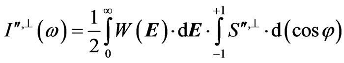 (19)
(19)
where
 ;
; (20)
(20)
Formulas (19) and (20) define the spectral line broadened by the electrons and the ions in presence of the uniform magnetic field  for all the observation directions
 :
:
 (21)
(21)
5. Dynamics and the Fluctuation Frequency Model
The method of the frequency fluctuation [5] stands on the idea that a quantal system in an electric field is as a fictious system which consists of a set of two-level transitions (dressed by the field). The field fluctuations induce a stochastic interference process between these transitions. At first step we must to construct all the possible transitions of the fictious system in the quasi-static approximation. This leads to write the evolution operator  corresponding to a given configuration as:
 (22)
(22)
averaged on the electric field, it can be written as:
 (23)
(23)
For one configuration of  and
and , the intensity with the help of (15) becomes:
or by using the Liouville representation:
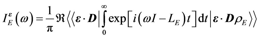 (24)
(24)
or after making the integral over t:
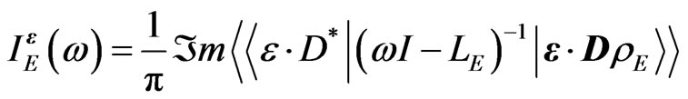 (25)
(25)
where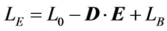 .
.
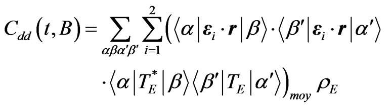
The diagonalization of the operator in (25) via the unitary matrix ME allows us to write the intensity as:
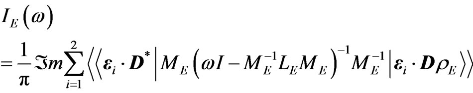 (26)
(26)
and
 (27)
(27)
where  and
and  are given by the above formula. Each term in the inner product (26) can be written as:
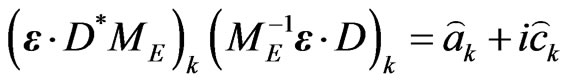 (28)
(28)
with a complex frequency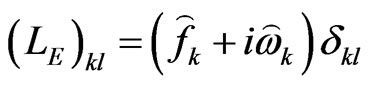 . Let be N the number of all terms in (26), then:
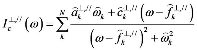 (29)
(29)
Here we have used the polarization towards  and the observation is parallel or perpendicular to the magnetic field.
6. Conclusion
In the presence of a magnetic field the emitted light by plasma is polarized. The line shape thus depends on the observation direction and the electric field direction relative to the magnetic field. This dependency complicates the calculation because the assumption of isotropic plasma is an approximation which is no longer valid in the presence of a magnetic field. We therefore fixed a direction of observation and considered all possible directions of the ionic field. The different steps of our calculation for solving this problem have been presented using the frequency fluctuation model to obtain the parallel and perpendicular intensities of the emitted radiation.
REFERENCES
- L. Landau and E. Liftchitz, “Quantum Electrodynamics, ‘Theoretical Physics’ Volume,” Mir Éd., Moscou, 1989.
- M. Baranger, “HGeneral Impact Theory of Pressure BroadeningH,” Physical Review, Vol. 112, No. 3, 1958, p. 855. HHUUdoi:10.1103/PhysRev.112.855UU
- K. Touati, “Spectroscopic Analysis of Plasma in the Presence of a Magnetic Field,” Doctoral Thesis, University of Provence, Marseille, 2003.
- Nguyen-Hoe, H.-W. Drawin and L. Herman, “Effect of a Uniform Magnetic Field on the Line Profiles of the Hydrogen,” Journal of Quantitative Spectroscopy and Transfer Radiation, Vol. 7, No. 3, 1967, p. 429.
- B. Talin, A. Calisti, L. Godbert, R. Stamm and R. W. Lee, “Frequency-Fluctuation Model for Line Shape Calculation in Plasma Spectroscopy,” Physical Review A, Vol. 51, No. 3, 1995, p. 8.
NOTES
*Corresponding author.