Applied Mathematics
Vol.08 No.05(2017), Article ID:76402,22 pages
10.4236/am.2017.85054
Time-Dependent Contaminant Transport in Ventilating Air from a Moving Source
George L. Danko, William Asante
University of Nevada, Reno, USA

Copyright © 2017 by authors and Scientific Research Publishing Inc.
This work is licensed under the Creative Commons Attribution International License (CC BY 4.0).
http://creativecommons.org/licenses/by/4.0/


Received: April 11, 2017; Accepted: May 21, 2017; Published: May 24, 2017
ABSTRACT
A new method which combines the Eulerian, fixed control volume with a moving, Lagrangean flow channel is described for the solution of the conjugate, advection-diffusion problem for modeling transport processes of contaminant species. The transport model is presented as a conservative mass balance equation in a state-flux, species transport form in the space-time domain. A fully-implicit, general solution scheme is formulated with matrix operators in the space-time domain. The particular solutions for specific initial and boundary conditions and source term are constructed with the help of a single, inverse matrix operator, A−1, which has to be calculated only once for all possible particular problems. Although A−1 involves a large number constants, all are independent from the initial, boundary, and source term input vectors. The multi-level, state-flux, space-time (SFST) scheme brings a significant computational acceleration since A−1 has to be calculated only once, such as in mine ventilation cases involving long drifts with constant air flow velocities. Such application is shown in an example for analyzing the transport and concentration distributions of diesel particulate matter (DPM) in the ventilation air at the working area with the interactions between ventilation and a moving diesel loading machine. Comparison between simulation and in situ DPM monitoring results suggests that reliable evaluation of average exposure of DPM to mine workers may be accomplished directly from tailpipe DPM emission data, ventilation air velocity, and mine geometry with the use of the SFST model even in a highly dynamic working area, potentially reducing the need for real-time DPM monitoring.
Keywords:
DPM Concentration, Species Transport, Numerical Modeling

1. Introduction
The transport of contaminant species by the moving air is of great importance in the natural atmosphere as well as in the built environment. Concentration of harmful chemical components or dust particles negatively affects health and safety of humans as well as the biosphere and must be controlled. Specific interest is of concentration distribution spread in space and with time originating from contaminant sources. Analysis, numerical model simulation and measurement are often needed to understand the transport of contaminant species for checking the concentration against regulatory compliance.
The transport mechanism of contaminants is complex involving advection, diffusion, dispersion, convection and accumulation in the moving air. Further complexity is added if the contaminant source is moving relative to the flow of air. Such problems are encountered in transportation tunnels, congested cities, and underground mines. Fick’s second law may serve as the fundamental component of the governing equations [1] [2] , but the formulation is based on the Eulerian, fixed control volume approach which requires fine spatial discretization. In the case of advection and diffusion, the Courant number, Cu, must be kept at Cu = 1 for accurate prediction from time-dependent simulation [3] [4] [5] . In case of moving source and independently moving air, the grid selection must be further constrained. The resulting solution in the form of a CFD (Com- putational Fluid Dynamics) model [6] [7] often require millions of spatial grid elements in sub-meter, or even micrometer size and of corresponding time steps in seconds, or down to even shorter temporal divisions.
A new method for modeling transport processes has been introduced that combines the Eulerian, fixed control volume with a moving, Lagrangean flow channel for a solution scheme for advection-diffusion problems [5] . The method promises a reduced grid sensitivity due to the intrinsic Cu = 1 condition built into the solution. The method, which can be used for the simulation of macroscopic flow, heat, and momentum transport, is briefly described here for contaminant transport studies. An example is provided for studying diesel emission variation in a ventilated underground working area with a moving loader machine. The numerical simulation results are compared with measurement data collected with stationary as well as moving sensors. The results are discussed and conclusions are drawn from the exercise.
2. Eulerian Balance Equation with Lagrangean Internal Transport
The general balance equation for advection, diffusion, dispersion, convection and accumulation of species e in the moving air is described in [5] in a stationary Eulerian volume V, swept with a Lagrangean flow channel of advection volume Va. The notations are shown in Figure 1 with a stagnant volume space as V-Va, filled by eddies, but with no net advection transport. The advection flux density component, qa flows as a Lagrangean wave front traveling at velocity v from Ain through Aout.
The transport balance equation for species e in the advection volume is [5] :
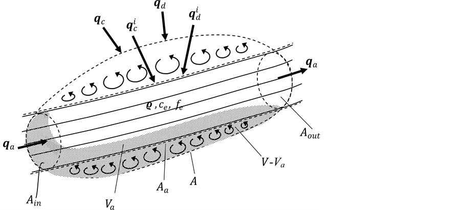
Figure 1. Control volume and surface for advection, convection, diffusion and accumulation (Reprinted from [5] with permission from Springer).
(1)
In (1), is advective mass flux density of species e; is the average travel time of the advective fluidoriginating from ; is the sum of diffusion, dispersion and convection of e across area, A; and are the densities of e and the bulk flow, respectively, and is the source term for species e.
Integral Equation (1) may be written in a finite difference form using finite volume and surface elements. With the introduction of the mass fraction variable, for species e, a State-Flux (SF) model is formulated in which the state, is the driving force for the transported mass flux density of species e [5] . The SF model is derived directly from (1), substituting volume
; stagnant volume ; and advection channel cross section surface. Note that the advection travel time, the spatial division, and flow velocity must obey the relationship , that is,
, for the validity of (1), where Cu is the Courant number [5] .
The sum of the first and second flux terms in (1) gives the advective flux driven by mass fraction difference, , where i and i + 1 denotes the input and the output points, respectively [5] :
(2)
The third term in (1) gives the difference of the flux by diffusion and convection (if applicable) driven by mass fraction differences, and :
(3)
The fourth term in (1) is the accumulation of the substance flux, proportional to the mass fraction change over the time period:
(4)
Note that the accumulation term is reduced to the stagnant volume only,
The right side of (1) expresses the source term of species e in control volume V:
(5)
Choosing a unit advective admittance, , the three transport admittances and the source term in (2)-(5) can be reduced to two, non-dimensional parameters, and , and a cell source term, , following [5] :
(6)
The reciprocal of the term in Equations (6) is recognized as the multiple of the Reynolds, Re, and Schmidt, Sc, numbers, two basic, non-dimen- sional parameters of transport processes [1] :
(7)
The normalized, finite difference form of (2) with the use of (6) and (7) constitutes the SF network equation for a network branch between nodes i − 1 and i, however, with the connection to node i + 1 also due to diffusion, dispersion, and convection [5] :
(8)
Note that the condition of validity of (8) is the unity of the Courant number, .
Assuming a homogeneous flow and transport field with constant material properties and transport coefficients, the SF network Equation (8) can be applied to a series of finite volume cells connected together. A fully implicit in space, time-marching in time solution scheme may be used for solving a set of network equations [5] . The time-marching step must be selected as . A multiple time step, fully implicit, State-flux, Space-Time (SFST) solution scheme can also be constructed offering a closed-form, operator solution for the conjugate advection, convection and diffusion-dispersion problem [5] .
3. A Fully Implicit, SFST Numerical Solution
A fully-implicit transport network solution is given in [5] using Equation (8) at

Figure 2. Substance transport network with explicit spatial and temporal grids (v > 0). (Reprinted from [5] with permission from Springer).
all the nodes and Equations (6) everywhere at the branches of a high-density internal grid. The transport network for such a multiple-level implicit scheme with inter-connected spatial and temporal grids is shown in Figure 2.
The boundary nodes with known driving potentials at time steps are separated from the active nodes of unknown potentials along spatial divisions. The advective transport connections between consecutive time levels are separated by potential followers, in order to provide the correct initial state values from time n − 1 to time n, affecting the substance flux density balance only at time n, but not at time n − 1. The initial potentials are established from time-step to time-step with no feedback flux effect from future time. The size of the network model to be solved simultaneously is (N ´ M)2.
It is shown that the solution can be expressed in a matrix-vector form with a five-diagonal admittance matrix, A, [5] . Out of the five diagonals, there is a triple-diagonal strip matrix symmetric around the main diagonal, stretching to the size of (N ´ M)2. In addition, there are two off-diagonal lines to include transport connections from the previous time interval. One off-diagonal line models the advection connections for each time step with the time-shifted potentials in the new A matrix, with . The other off-diagonal line includes the accumulation connections for the stagnant volume, for each internal time step. The five-diagonal matrix,#Math_43# for a positive, left-to-right, v > 0 velocity is [5] :
(9)
For a right-to-left, va < 0 velocity, the advection connections are transposed:
(10)
Matrix A may be viewed as a composite array of M ´ M sub-matrices, ai,j, i.e., :
(11)
In (11), the diagonal sub-matrices, are N × N in size, . The ai,i elements constitute triple-diagonal sub-matrices:
(12)
The off-diagonal sub-matrices, are mainly zeros. For left-to-right, v > 0 velocity, the non-zero off-diagonal sub-matrices for are:
(13)
The advection connections are transposed for the right-to-left, v < 0 velocity in the off-diagonal elements, as follows for :
(14)
For all other sub-matrixes, not defined by (12) through (14), are null matrices, ai,j = {0}. Consequently, A(i,j) is dominantly a sparse matrix.
Although the structure of the matrix operators are different for v > 0 from v < 0 velocity directions, the notations are simplified and applied for left-to-right, v > 0 velocity, shown in Figure 2.
For simplicity, sub-matrix notations are used for the upward and downward boundary condition vectors, BUd, BUa and BDd, as well as the initial condition vector, IC. The boundary and initial condition sub-vectors in the matrix-vector balance equation have to be all in the length of N × M, filling them with zeros where no connections are defined in the network of Figure 2, and keeping their non-zero value at the active connections. Using the notation of , , and , respectively, the boundary vector elements are:
(15)
(16)
(17)
(18)
The unknown mass fraction vector, , is also used in sub-vectors form of :
(19)
Distributed substance source for each node in Figure 2 may be included, varying with space and time. The source term in sub-vector form is:
(20)
The balance equation of the SF network of Figure 2 is now written in sub-matrix notation:
(21)
The simultaneous solution for the entire mass fraction field with space and time is:
(22)
All sub-vectors except for the distributed source term vector are substantially sparse in (22). It is possible to eliminate the zero elements from the terms on the left side of (22) and to return to the full initial and boundary condition vectors [5] . The source term is also reduced to an M-element Fs vector by either accepting the average of the nodal sources along each line, or sampling the values of the Fi(j) vector along a desired trajectory, e.g., along a moving source, in the x-t space within the cell domain. With these simplifications by algebra, a new matrix-vector equation is obtained with matrices of MN rows and M columns, with still full expression for all MN mass fraction values, but in need of M-vectors only on the right side [5] :
(23)
In (23), five different coefficient matrices emerged with the definitions as follow:
The coefficient matrices in (23) and (24) all have rows, but the number of columns is N in and M in all the other four matrices. Therefore, the full matrices in (23) are different from each other; and all have much smaller size that A−1 in (22).
Note that the last row in each matrix in Equation (23) is not sparse and may involve a large number constants, carrying all of information necessary for expressing the solution the conjugate advective and diffusive transport in the ST domain with matrix operators, all independent from the IC, BU, and FS input vectors. At the same time, the multi-level scheme brings a significant computational acceleration if A−1 has to be calculated only once, such as in mine ventilation for each long drift with a constant, advection velocity. Such application is shown in an example as follows.
4. Application Example of the SFST Model with Moving Source Term
Based on an underground mine experiment [9] , an example of the method is described for contaminant concentration distribution in the ventilating air in a mine drift. A mine haulage route for a diesel load-haul-dump (LHD) machine in the experiment is shown in Figure 3. Diesel particulate matter (DPM), a contaminant is modeled as it is transported in the ventilating air by advection and dispersion, emitted from the tail pipe as a moving source of the engine. The machine travels back and forth along the specified route, continuously repeating a loading cycle.
In order to capture the tailpipe DPM contaminants from the exhaust fumes directly, two sampling sensors were placed 2.1 m away from the tailpipe. Three pairs of stationary sensors were placed, two at each location at three different points on the wall, marked as m1, m2, and m3 at 3.1 m, 41 m, and 78 m from the loading area to measure the DPM concentration in the ventilating air.

Figure 3. Plan view of mine drift.
The ventilating air enters the mine drift at the mid-section and splits into two directions. The left side (LS) drift segment, 78 m long, leads to the loading zone. The right side (RS) segment, 241 m long, stretches to the dumpling zone. The two drift segments require two separate DPM transport models. The connection between the two model sections is the loading machine crossing from one to the other in a cyclic manner. The diesel exhaust source of the loading machine moves with a travel velocity of in either the LS or RS drift section. The airflow velocity of is also the same in both the LS and the RS segments.
Figure 4 depicts the cycle time diagram for the loading machine and the airflow directions. The moving sensor measuring concentration is placed 2.1 m behind the moving point source and modeled independently in the two separate sections. The point where the air flow splits into two opposite directions to the left and right sections is used as a reference point for background concentration. The DPM concentration of 90 μg/m3, measured as an incoming value at the intake air from the other areas of the mine, is used in the example as a constant additive to the zero concentration level in the numerical model. The concentration from the moving sensors on the loading machine is modeled by sampling the spatial concentration from the SFST solution at an offset of 2.1 m distance from the exhaust point of the tailpipe.
The airflow directions and the spread of the tailpipe exhaust fumes are illustrated in Figure 5 as the machine travels in the haulage drift in and out of the LS and the RS drift segments. The efficiency of catching the DPM from the exhaust plumes by the moving sensor depends on the direction of the movement of the machine as well as the air flow direction relative to the machine.
A fine spacial mesh of 1.3 m and 1 second of temporal discretization is used in both the LS and RS for the numerical models, satisfying the condition for the Courant number of Cu = 1.3/1.3 = 1. The model is setup using the geometry of

Figure 4. Cycle time diagram for the loading machine and the airflow directions.
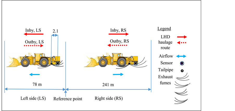
Figure 5. Airflow directions and spread of tailpipe exhaust fumes as a result of the LHD machine movment.
the mine experiment. Accordingly, the N and M divisions in the spatial and temporal meshes are N = 60, M = 162 for the LS and N = 186, M = 258 for the RS model segments.
Figure 6 and Figure 7 show the machine velocity versus distance diagram per cycle and machine velocity versus time diagram, respectively. The source term is determined from measured diesel fuel use for the haulage and the tailpie emis- sion data [9] . The DPM concentration source term entering the air flow from the tailpipein the model is 1000 μg/kg/s, determined based on LHD machine data. Note that the moving point source is a cumulative transport term that cannot be converted directly into a mass fraction (or volumetric concentration) in the moving air stream without considering the advetive, dispersive, and accumulation components. Assuming no stagnant volume in the drift cross section (S = 0), no dispersion, (D = 0), and near-zero advective air flow velocity, (such as that
), the source term would continuously increase the contaminant mass fraction according to as seen from Equation (8).
Therefore, the mass fraction (and the corresponding volumetric concentration) would both increase linearly with time to infinity.
The transient mass concentration distributions are of interest at various moving and fixed points: at the moving source i.e., at the exhaust tailpipe; at a sensor fastened on the machine with an offset of 2.1 m behind the tailpipe and at three fixed locations in the airway. The fixed locations are: at x = L/25, close to the en-

Figure 6. Machine velocity versus distance diagram for a full haulage cycle.

Figure 7. Machine velocity versus time diagram.
trance to the tunnel; at x = L/2; and at x = L.
Matrix A in (11) and matrices in (23) are calculated with N = 60 and M = 162 for the LS, and N = 186 and M = 258 for the RS drift segments, respectively. The size of A (and A−1) in the operator solution are 9720 × 9720 in the LS and 47,988 × 47,988 in the RS models, both calculated only once in the examples for each dispersion coefficient. The dispersion coefficients is calculated as D = 2.5 m2/s for turbulent pipe flow in reference to Taylor’s results [8] , but two lower values of 0.05 m2/s and 0.5 m2/s are also used for sensitivity checks in the example. Zero initial and boundary values, i.e., IC = BU = BD = 0, are assumed in the Eulerian domain. The source points are defined along the traveling trajectory of the machine over the space-time plane intersecting or passing by minimum distance from M grid points which now represent the Lagrangean model domain. The mass concentration values are calculated from the full ST solution of (23), applied separately to the LS and RS drift segments. The spatial and temporal concentration values for the stationary and moving sensors; as well as the tailpipe of the LHD are determined from the full ST solutions by sampling the data sets obtained for the LS and RS drift segments.
The full ST solution is shown in Figure 8(a) and Figure 8(b). Both figures depict the mass concentration field with D = 2.5 m2/s. For graphical purposes, the large model size is reduced by sampling only every 10th of the DPM mass fraction values, converted to the more convenient concentration units.
The desired solution for concentration both at fixed as well as at the moving points is expressed from the full solution for the entire space-time plane at the space-time grid points. Since both the result and source vectors have M elements, the solution equation is always in the form of:
(25)
where is calculated from the common matrix operator by multiplication with individual sampling matrices defined in relations (24) for different model resultant solutions, R, according to the selection of the sampled points in the LS and RH segments along the characteristics lines of the traveling machine, shown in Figure 4.
Three different dispersion coefficients, 0.05 m2/s, 0.5 m2/s, and 2.5 m2/s are tested with the model for three independent simulations. The goal is to assess the effect of dispersion on the concentration predicted by the model. The simulated average concentrations are calculated for the moving sensor, as well as the stationary sensors. These values are used to calculate the cycle average concentrations.
Figure 9 and Figure 10 show the DPM concentration for the LHD tailpipe and the DPM moving sensors for the LS and RH segments, respectively. Figure 11 depicts the concentrations for the fixed locations sensors with D = 0.05 m2/s. Two higher dispersion coefficients are used in the simulations for sensitivity examination with D = 0.5 m2/s and D = 2.5 m2/s. For D = 0.5 m2/s, the DPM concentration for the LHD tailpipe and the DPM moving sensors are illustrated in Figure 12 and Figure 13 for the LS and RH segments, respectively. The concentration for the fixed location sensors are shown in Figure 14 for D = 0.5 m2/s. Figure 15 and Figure 16 depict the DPM concentration for the LHD tailpipe and the DPM moving sensors for the LS and RH segments, respectively, assuming a dispersion coefficient of D = 2.5 m2/s; the corresponding concentrations for the stationary sensors are shown in Figure 17.
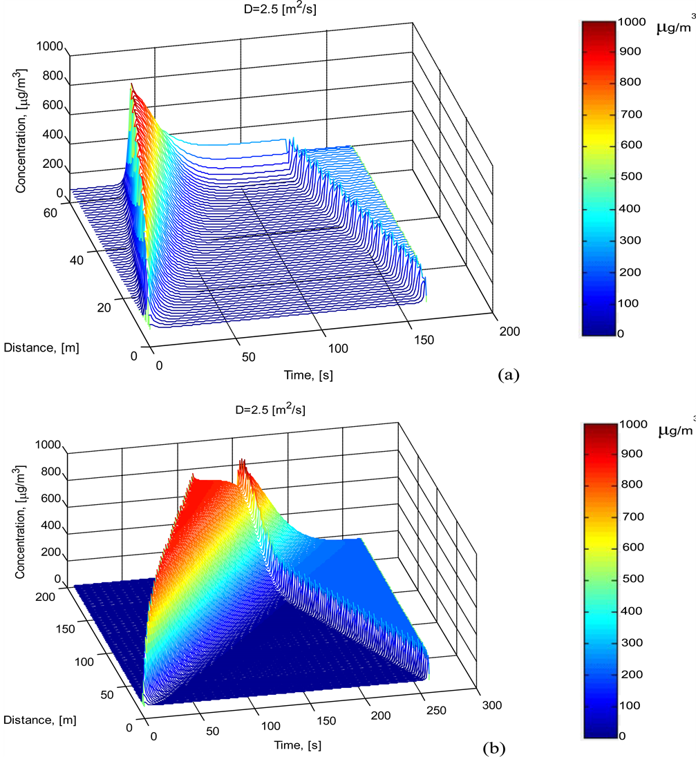
Figure 8. Full SFST solution with D = 2.5 m2/s; (a) left side, LS; (b) right side, RS.
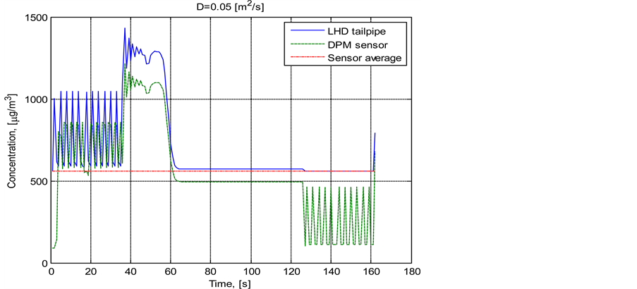
Figure 9. Sampled mass concentrations at moving points on the LS drift segment with D = 0.05 m2/s.

Figure 10. Sampled mass concentrations at moving points on the RS drift segment with D = 0.05 m2/s.

Figure 11. Sampled mass concentrations at fixed points on the LS drift segment with D = 0.05 m2/s.

Figure 12. Sampled mass concentrations at moving points on the LS drift segment with D = 0.5 m2/s.

Figure 13. Sampled mass concentrations at moving points on the RS drift segment with D = 0.5 m2/s.

Figure 14. Sampled mass concentrations at fixed points on the LS drift segment with D = 0.5 m2/s.

Figure 15. Sampled mass concentrations at moving points on the LS drift segment with D = 2.5 m2/s.

Figure 16. Sampled mass concentrations at moving points on the RS drift segment with D = 2.5 m2/s.

Figure 17. Sampled mass concentrations at fixed points on the LS drift segment with D = 2.5 m2/s.
5. Discussion of the SFST Method and the Results in the Example
The SFST solution for a moving substance source is given in a Eulerian domain overlaid with a Lagrangean space. The particular solutions for the initial and boundary conditions and source term are constructed with the help of a matrix operator, A−1, which has to be calculated only once for the LS and the RS drift segment for all particular, initial and boundary problems and even with the moving DPM source. The A−1 matrix operators would remain valid for any other movement characteristics of the pollutant source term, however, the sampling matrices in (23) and (24) would have to change.
The method is advantageous to use where the air flow direction and velocity in the underground drifts are known, and the iA = A−1 can be conveniently pre-calculated. Such a case is often found in underground mines with constant ventilation and long time periods of continuous loading operations such as in the application example for diesel emission measurement evaluation.
The results for the three independent simulations performed at two separate sections such as LS and RS of the mine drift using the three different dispersion coefficient are delineated as follows.
5.1. LS, LHD Tailpipe and Moving Sensor Concentration Variations
It is interesting to observe that the DPM concentration at the tailpipe exit point over the entire length of the inby section show a saw tooth-shape fluctuation. With low dispersion (D = 0.05 m2/s, Figure 9), the amplitude of fluctuation does not change due to the fact that the machine always encounters a portion of fresh air at with background concentration at the time of entering a new airway section of which is then charged by the source term resulting in a near-constant (and corresponding volumetric concentration) change. Since the speed of the LHD machine is higher than that of the air and the machine does not travel perfectly together with the same discrete air volume (however, part of the previous air section is still connected during a time interval), the concentration at the next section starts again at a lower concentration which is interestingly higher than the background concentration due to the near-instantaneous introduction of pollutant source to the control volume upon arrival at at the tailpipe exit point. It is assuring to observe that when the transport connection is spread to a larger volume with increased dispersion (Figure 12, Figure 15), the DPM concentration shifts toward starting from the background concentration, and the amplitude of the saw tooth variation is decreasing.
The DPM concentration is shown to be sensed by the moving sensor very well over the entire length of the inby section in Figure 9, due to the favorable LHD movement direction for the exhaust plume in this section as illustrated in Figure 5, with the DPM sensor in the plume behind the tailpipe. It is assuring to see that the starting concentration of the moving sensor is at the background value and that the amplitude of the saw tooth variation is smaller, due to dispersion over a larger distance of the offset of 2.1 m that is larger than the value of m. With increased dispersion shown in Figure 12 and Figure 15, the DPM concentration from the moving sensor is getting smoother following very well the concentration of the tailpipe emission curve.
At the loading point, the LHD and the moving sensor are stationary. As shown in Figure 9, the concentration gradually accumulates with time due to the continuous pollutant mass source as well as the arrival of the polluted air that is left behind the faster-moving machine. With increased dispersion shown in Figure 12 and Figure 15, the DPM concentration from the moving sensor at the loading point is getting lower and smoother, but always following very well the concentration of the tailpipe emission.
The DPM concentration at the tailpipe and the moving sensor in the LS drift section during the outby travel of the LHD are very different from that of the inby travel, as seen in Figure 9. The DPM concentration at the tailpipe appears to be smooth due to traveling against the air flow with low dispersion. For the concentration of the moving sensors, three processes compete: 1) the increase of the concentration in the section due to the DPM source which travels against the counter-flow of the air; 2) the instantaneous dispersion along the drift, spreading the concentration from the tailpipe; and 3) the 2.1 m offset of the moving sensor stretching into the next section at background concentration. Consequently, a fluctuation is seen showing periodic variations between the background and tailpipe concentrations, the frequency depending on the grid alignment with the traveling characteristics of the sensor during sampling the discretized concentration profile.
5.2. RS, LHD Tailpipe and Moving Sensor Concentration Variations
A similar phenomena as explained in the LS drift section are observed for the DPM concentration at the tailpipe exit point for the inby and outby sections of the RS drift section shown in Figure 10, Figure 13, and Figure 16 with dispersion coefficients of D = 0.05 m2/s, D = 0.5 m2/s, and D = 2.5 m2/s, respectively. However, the difference is that, unlike the LS, the DPM concentration is shown not to be sensed by the moving sensor very well over the entire length of the inby section in Figure 10, Figure 13, and Figure 16. For the outby section, the moving sensor concentration slightly increases at the start of the section due to the LHD meeting the fume that is left behind by the tailpipe source as a result of the short dumping time and the late arrival time of the air flow. However, the concentration of the moving sensor immediately reduces to the background concertation at the arrival of the airflow, diluting the plume. The significant reduction in concentration in Figure 10 can be attributed to the unfavorable LHD movement direction relative to the sensor (with the DPM sensor in the plume being behind the tailpipe) for both inby and outby sections as illustrated in Figure 5.
Similar trends can be seen with increased dispersion coefficients in Figure 13 and Figure 16, albeit the higher dispersions appear to connect the moving sensor to the tailpipe better, elevating concentration levels.
At the dumping point, the LHD and the moving sensor are stationary. As shown in Figure 10, the concentration gradually accumulates with time due to the continuous pollutant mass source as well as the arrival of the polluted air left behind the moving machine. With increased dispersions in Figure 13 and Figure 16, the DPM concentration from the moving sensor at the dumping point is getting lower and smoother, but always following very well the concentration of the tailpipe emission.
5.3. LS, Stationary Drift Location Sensors
The stationary drift sensors at the LS drift section show increasing concentrations in the inby section in Figure 11 as the LHD moves from the reference point to the loading point. This is due to the lower velocity of the air than that of the tailpipe DPM source. The sensors show afluctuation in concentration with a reduced amplitude in the outby section in Figure 11 upon the return of the LHD. This is caused by the counter-direction of the air flow to the LHD and the phenomena of the sampling effects upon the concentration variations with moving air and source explained in the foregoing. The air mixes with the source concentration and dilutes it. During loading, the concentration of the fixed drift sensors are significantly reduced towards the background concentration due to the direct removal of the tailpipe source by the air. The width of the concentration pulses for the sensors at points 3, 2, and 1 located at 78 m, 41 m, and 3.1 m away from the air intake point increase as the distance gets further from the point at background concentration. The reason for this is the different duration of the exposure to the pollutant source. With D = 0.05 m2/s in Figure 11, the concentration pulses are nearly rectangular. With increased dispersions shown in Figure 14 and Figure 17, the DPM concentrations from the fixed sensors are taking an asymmetrical shape with sharp increase and a slow descent referred to as “heavy tail” in the transport literature for contaminants.
5.4. Cycle Weighted Averages (CWA) and Comparison of Model Results to Measured Data
Part of the process of evaluating the concentrations at the moving and stationary sensors is to calculate time-averaged values for the haulage cycles in both the LS and RS drift sections. These average values are depicted in Figure 9 through Figure 17. Furthermore, a cycle averaging and weighting method is used to process the average DPM concentration data from the model results shown in Figure 9 through Figure 17. The calculated cycle weighted averages (CWA) using weight factors of 162 seconds for LS and 258 seconds for the RS is as follows:
(26)
where:
LSav = Left side average concentration (μg/m3),
RSav = Right side average concentration (μg/m3).
The RSav used for the stationary sensors is 90 μg/m3, which is the background concentration entered into the model. Table 1 summarizes the CWA obtained from the SFST model for the different dispersion coefficients.
As seen in Table 1, different dispersion coefficients in the model do not have much effect on the average concentration values. This is in spite of the observed changes in the varying shape of concentration spreads in Figure 9 through Figure 17, such as less spread and higher peak concentration values for a low dispersion coefficient due to little mixing of the contaminant with air; and better spread and lower peak concentration values with high dispersion coefficients. However, the time-averaged values are not significantly affected, a favorable outcome for the otherwise uncertain parameter, D, in the mining environment.
The results of the SFST model are compared with in situ DPM in situ measurements performed at an underground mine [9] . The DPM measurement results are summarized in Table 2.
Comparison of DPM measurement data with the SFST model simulation results is shown in Table 3 for different dispersion coefficients. As seen, the dispersion coefficient values have a relatively minor effect on the average concentrations. The concentration values predicted by the SFST model for all different dispersion coefficients are in very good agreement with the measured concentration values from the mine. The model error selecting the D = 0.5 m2/s, dispersion coefficient relative to the measured concentration is 5.8% for moving sensor and less than 10% for the average of the data from three stationary sensor locations.
The numerical simulation and the comparison with in situ measurement results prove that the average DPM concentration in the air at any area in the mine

Table 1. Summary of CWA from the SFST model for different dispersion coefficients.
Table 2. DPM measurement results.
Table 3. Comparison of measurement data with model results using different dispersion coefficients.
can be predicted from the DPM mass transport model using the SFST simulation. The DPM source term from the tailpipe DPM concentration and their fuel consumption data can be evaluated as an input to the SFST simulation model. The mass balance and transport network modeling method ensures a cost effective and accurate way of predicting average DPM concentrations in underground mines, reducing the need for real-time monitoring for appropriate ventilation design.
6. Conclusions
・ A new, powerful, fully-implicit SFST solution is applied for interpreting mea- surement results for DPM contaminant concentration variations from a moving machine in an underground mine.
・ The mathematical model provides a link between the time-averaged and the peak DPM concentration values at the tailpipe.
・ Very good match was obtained for all three drift stationary sensors as well as the moving sensor with D = 0.05, 0.5 and 2.5 m2/s between in situ measurement results and SFST model simulation.
・ The DPM concentration variations with location and time in the air of the mine can be predicted from the known tailpipe DPM concentration from machine smog tests and the fuel consumption of the diesel machine.
・ Therefore, the mathematical model may be used to evaluate the average concentration exposure value of the DPM for compliance analysis without real-time, complicated DPM measurements, relying basically on tailpipe smog test, fuel consumption and the SFST contaminant transport model, incorporated in the mine ventilation model.
・ With the simulation of total, accumulated DPM concentration at the working area, mining companies will be able to implement the right ventilation strategies to reduce or eliminate harmful DPM exposure to mine workers.
Acknowledgements
A research support grant from the National Institute of Occupational Safety and Health, USA (NIOSH) is thankfully acknowledged.
Cite this paper
Danko, G.L. and Asante, W. (2017) Time-Dependent Contaminant Transport in Ventilating Air from a Moving Source. Applied Mathematics, 8, 671-692. https://doi.org/10.4236/am.2017.85054
References
- 1. Bird, R.B., Steward, W.E. and Lightfoot, E.N. (1960) Transport Phenomena. John Wiley and Sons, New York.
- 2. Welty, J.R., Wicks, C.E. and Wilson, R.E. (1984) Fundamentals of Momentum, Heat and Mass Transfer. 3rd Edition, John Wiley and Sons, New York.
- 3. Le Veque, R.D. (2002) Finite Volume Methods for Hyperbolic Problems. Cambridge University Press, Cambridge. https://doi.org/10.1017/CBO9780511791253
- 4. Peacemen, D.W. (1977) Fundamentals of Numerical Reservoir Simulation. Elsevier Scienticic, New York, 65-82.
- 5. Danko, G. (2016) Model Elements and Network Solutions of Heat, Mass and Momentum Transport Processes. Springer-Verlag GmbH, Berlin. http://link.springer.com/book/10.1007%2F978-3-662-52931-7
- 6. Fluent 5.5, ANSYS (1997) Copyright Fluent Inc., Lebanon.
- 7. Cradle (2012) Thermofluid Analysis System with Unstructured Mesh Generator SC/Tetra Version 10 User’s Guide. Software Cradle Co., Ltd.
- 8. Taylor, G. (1954) The Dispersion of Matter in Turbulent Flow through a Pipe. Proceedings of the Royal Society of London, 223, 446-468. https://doi.org/10.1098/rspa.1954.0130
- 9. Asante, W. (2014) Mine-Wide Diesel Particulate Matter (DPM) Monitoring Applications. MS Thesis, University of Nevada, Reno, 1-89.