Applied Mathematics
Vol.06 No.06(2015), Article ID:56863,11 pages
10.4236/am.2015.66089
Solving Doubly Bordered Tridiagonal Linear Systems via Partition
Moawwad El-Mikkawy1*, Mohammed El-Shehawy2, Nermeen Shehab2
1Mathematics Department, Faculty of Science, Mansoura University, Mansoura, Egypt
2Mathematics Department, Faculty of Science, Damietta University, Egypt
Email: *m_elmikkawy@yahoo.com, melshehawey@yahoo.com, nermeen_shehab87@yahoo.com
Copyright © 2015 by authors and Scientific Research Publishing Inc.
This work is licensed under the Creative Commons Attribution International License (CC BY).
http://creativecommons.org/licenses/by/4.0/


Received 27 April 2015; accepted 30 May 2015; published 2 June 2015
ABSTRACT
This paper presents new numeric and symbolic algorithms for solving doubly bordered tridiagonal linear system. The proposed algorithms are derived using partition together with UL factorization. Inversion algorithm for doubly bordered tridiagonal matrix is also considered based on the Sherman-Morrison-Woodbury formula. The algorithms are implemented using the computer algebra system, MAPLE. Some illustrative examples are given.
Keywords:
Doubly Bordered Tridiagonal Matrices, UL Factorization, Block Matrices, Computer Algebra Systems, Sherman-Morrison-Woodbury Formula

1. Introduction
Linear systems are among the most important and common problems encountered in scientific computing. The whole range of technical problems leads to the solution of systems of linear equations. The first step in numerical solution of many problems is a choice of an appropriate algorithm.
Throughout this paper the word, “simplify”, means simplify the expression under consideration to its simplest rational form. The abbreviation DBT refers to doubly bordered tridiagonal.
The main objective of the current paper is to construct efficient algorithms for solving DBT linear system of the form:
 (1)
(1)
where the coefficient matrix A is a DBT matrix with the special structure of the partitioned form

 and,.
and,.
Such systems arise in many scientific and engineering applications when considering certain partial differential equations and spline approximation. For more details see, for instance [1] -[5] . It is worth noting that in [6] , the authors solved the system (1) via transformation method. In this paper, we are going to solve the system under consideration via partition.
The linear system (1) can also be written in block form as follows:
 (3)
(3)
where
 (4)
(4)
is a  block matrix,
  ,
, 
 , and is
 tridiagonal matrix which is given by
 (5)
(5)
The present paper is organized as follows. In Section 2, we introduce some facts about tridiagonal matrices and a new recursive procedure for inverting this matrix is proposed. In Section 3, the UL factorization of DBT matrix is considered. Numeric and symbolic algorithms for evaluating DBT matrix determinant are constructed. Also a symbolic algorithm for computing the inverse of DBT matrix is developed using the Sherman-Morrison- Woodbury formula. Finally, the solution of the linear system whose coefficient matrix is of DBT matrix type is proposed. In Section 4, some illustrative examples are given.
2. Preliminaries and Basic Results
Tridiagonal matrices arise in many contexts in pure and applied mathematics. Also, they arise in many different theoretical fields, especially in applicative fields such as spline approximation, numerical analysis, ordinary and partial differential equations, solution of linear systems of equations, engineering, telecommunication system analysis, system identification, signal processing (e.g., speech decoding), partial differential equations and naturally linear algebra. See [1] - [4] . Research area on these types of matrices is very active and has recently attracted the attention of many researchers.
In many of these areas, inversions of tridiagonal matrices are necessary and different approaches are considered [7] - [10] in order to obtain such inverse. Some authors consider a general tridiagonal matrix of finite order and then describe the LU factorizations, determine the determinant and inverse of a tridiagonal matrix under certain conditions [1] , [2] and sometimes without any restrictive conditions [8] , [11] . The interested reader may refer to [12] - [23] .
The general tridiagonal matrix  takes the form
 (6)
(6)
in which  for
for .
.
When we consider the matrix T defined by (6), it is helpful to introduce the n quantities  as follows:
 (7)
(7)
Following [8] , we have the following result whose proof will be omitted for the sake of space requirement.
Theorem 2.1. The UL factorization of the matrix T in (6) is possible if  for each
 . In this case we have the following two UL factorizations:
 (8)
(8)
where
 (9)
(9)
and
 (10)
(10)
The following are two useful remarks:
Remark 1: The matrices  in (9) and (10) are related by
 (11)
(11)
and
 (12)
(12)
where
 (13)
(13)
Remark 2: If the UL factorization of the matrix T in (6) is possible, then we have:
 (14)
(14)
where  are given by (7). In other words, the matrix T is invertible as long as
 (15)
(15)
Now we are going to state the following result without proof.
Theorem 2.2. Let T be a non-singular tridiagonal matrix, given by (6), and let  then for
 we have
 (16)
(16)
where 
3. Doubly Bordered Triangular Matrix (DBT Matrix)
In this section, we are going to construct new numeric and symbolic algorithms to evaluate the determinant of a DBT matrix and to compute the inverse of such matrices. For these purposes it is advantageous to consider the UL factorization.
To factor the n × n DBT matrix A given in (2) into the product of an upper-triangular matrix  and a lower-triangular matrix
  in the form A = UL, we may proceed as follows
 (17)
(17)
where
 (18)
(18)
and
 (19)
(19)
Equation (17) can be written in block matrix form as follows:
 (20)
(20)
where ,
,  and
and  are the lower and upper triangular matrices of the tridiagonal matrix
  given in (5), respectively.
From (20), we see that the following equations are satisfied:
 (21)
(21)
 (22)
(22)
 (23)
(23)
and
 (24)
(24)
Solving (21), (22) and (23) for ,
,  and
and  yields:
 (25)
(25)
 (26)
(26)
and
 (27)
(27)
where
 (28)
(28)
3.1. Algorithms for Evaluating the Determinant of a DBT Matrix
The determinant of the matrix A in (2) can be computed using the following numeric algorithm.
Algorithm 3.1. A numeric algorithm for computing the determinant of a DBT matrix.
To compute the determinant of the DBT matrix in (2), we may proceed as follows:
INPUT: Order of the matrix, n and vectors a, d, b, h, v.
OUTPUT: The determinant of the matrix A in (2).
Step 1: Set .
.
Step 2: For i = n − 1, n − 2, …, 2 do
compute and simplify 
End do.
Step 3: Compute e1 using (27).
Step 4: 
As can be easily seen, Algorithm (3.1) breaks down if any ei = 0 for some . The following symbolic algorithm is developed in order to remove the case where the numeric algorithm fails.
Algorithm 3.2. A symbolic algorithm for computing the determinant of DBT matrix.
To compute the determinant of the DBT matrix in (2), we may proceed as follows:
INPUT: Order of the matrix, n and vectors a, d, b, h, v.
OUTPUT: The determinant of the matrix A in (2)
Step 1: Set . If
. If  then
then  End if. (t is just a symbolic name)
Step 2: For i = n − 1, n − 2, …, 2 do
compute and simplify:
 If
If  then
then  End if.
End do.
Step 3: Compute and simplify e1 using (27).
Step 4: Compute and simplify:

Step 5: Det (A) = p(0).
The Algorithm (3.2) will be referred to as DETGDBTRI algorithm.
3.2. Algorithm for Inverting DBT Matrix
In this sub-section, we are going to formulate a new symbolic algorithm for inverting the general DBT matrix based on the Sherman-Morrison-Woodbury formula.
A general DBT matrix can be written as following:
 (29)
(29)
Applying the Sherman-Morrison-Woodbury formula [13] to A gives
 (30)
(30)
Now we are ready to formulate the following symbolic algorithm for inverting the DBT matrix.
Algorithm 3.3. A symbolic algorithm to compute the inverse of a non-singular DBT matrix.
To invert a general DBT matrix (2), we may proceed as follows:
INPUT: The order of the matrix, n and the entries of the matrices T, U and V.
OUTPUT: The inverse of the DBT matrix A given in (2).
Step 1: Set . If
. If  then
then . (t is just a symbolic name)
Step 2: For  do
do
compute and simplify:
 . If
. If  then
then  End if
End do.
Step 3: Compute and simplify the elements of the inverse matrix  using (16).
Step 4: compute  using (30).
Step 5: Substitute t = 0 in all expressions of the matrix .
.
3.3. Solving Linear System of Equations of DBT Matrix Type
In this sub-section, we introduce different approaches for solving doubly bordered tridiagonal linear systems of the form (1).
The inverse matrix of the DBT matrix A introduced in (2) could be written in the block form as follows:
 (31)
(31)
where ,
,  and
and
Now, we can formulate our first algorithm for solving the linear systems of the form (1).
Algorithm 3.4. A first numeric algorithm for solving linear systems of DBT matrix type.
To solve a general bordered tridiagonal linear system of the form (1), we may proceed as follows:
INPUT: The entries of the matrix , the value of d1 and the vectors
 .
.
OUTPUT: The solution vector .
.
Step 1: Compute .
.
Step 2: Compute .
.
Step 3: The solution vector is .
.
As we can see, the computational cost of Algorithm (3.4) is .
.
The following algorithm depends on the UL factorization of the coefficient matrix A in (1), so it is more convenient to rewrite the linear system (1) as:
 (32)
(32)
To solve the linear system (32), it is equivalent to solve the two standard linear systems:
 (33)
(33)
and
 (34)
(34)
where  and
and .
.
Armed with the above results, we may formulate the following numeric algorithm:
Algorithm 3.5. A second numeric algorithm for solving linear systems of DBT matrix type.
To solve a general doubly bordered tridiagonal linear system of the form (1), we may proceed as follows:
INPUT: The components,  and
and .
.
OUTPUT: The solution vector  of the linear system in (1).
Step1: Use the algorithm (3.1) to check the non-singularity of the coefficient matrix A of the system (1).
Step2: If Det (A) = 0; then OUTPUT (‘no inverse exists’); STOP.
Step 3: Set .
.
Step 4: For  do
do
compute 
End do.
Step 5: Compute 
Step 6: Set .
.
Step 7: Compute 
For  do
do
compute 
End do.
Step 8: The solution vector 
To remove all cases in which Algorithm (3.5) fails, it is convenient to give the following symbolic version of the numeric algorithm described above.
Algorithm 3.6. A symbolic algorithm for solving linear systems of DBT matrix type.
To solve a general doubly bordered tridiagonal linear system of the form (1), we may proceed as follows:
INPUT: The components,  and
and .
.
OUTPUT: The solution vector  of the linear system in (1).
Step 1: Use the DETGDBTRI algorithm to compute .
.
Step 2: Use the DETGDBTRI algorithm to check the non-singularity of the coefficient matrix A of the system (1).
Step 3: If Det(A) = 0; then OUTPUT (‘no inverse exists’); STOP.
Step 4: Compute and simplify  using (25).
Step 5: Compute and simplify  using (26).
Step 6: Set .
.
Step 7: Compute and simplify  using (28).
Step 8: For  do
do
Compute and simplify:

End do
Step 9: Compute and simplify:

Step 10: Set .
.
Step 11: Compute and simplify:

For  do
do
Compute and simplify:
 .
.
End do.
Step 12: Substitute t = 0 in all expressions of the solution vector 
The computational cost of Algorithm (3.6) is  multiplications/divisions and
  additions/ subtractions. The Algorithm (3.6) will be referred to as DBTLSys algorithm.
4. Illustrative Examples
In this section we give four examples for the sake of illustration.
Example 4.1. Solve the following periodic tridiagonal linear system of size 12.
 (35)
(35)
Solution: we will solve this system as a DBT linear system where

By applying DBTLSys algorithm, we have
・ 
・ 
・ The solution vector is .
.
This result is in complete agreement with the result in [14] .
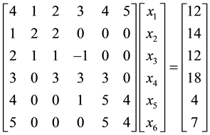
Example 4.2. Solve the following DBT linear system
 (36)
(36)
Solution: we have a DBT linear system with

By using DBTLSys algorithm we have
・ 

・ The solution vector is .
.
This result is in complete agreement with the result in [6] .
Example 4.3. Solve the following DBT linear system
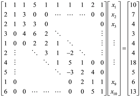 (37)
(37)
Solution: we have a DBT linear system with

By using DBTLSys algorithm we have
・ 
・ 
・ The solution vector is .
.
Example 4.4. Solve the following DBT linear system
 (38)
(38)
Solution: we have a DBT linear system with

By using DBTLSys algorithm we have
・ 
・ 
・ The solution vector is 
References
- Udala, A., Reedera, R., Velmrea, E. and Harrisonb, P. (2006) Comparison of Methods for Solving the Schrödinger Equation for Multiquantum Well Heterostructure Applications. Proceedings of the Estonian Academy of Sciences, Engineering, 12, 246-261.
- Pajic, S. (2007) Power System State Estimation and Contingency Constrained Optimal Power Flow―A Numerically Robust Implementation. Polytechnic Ins. [S.l.], Worcester.
- Mazilu, I., Mazilu, A.D. and Williams, H.T. (2012) Applications of Tridiagonal Matrices in Non-Equilibrium Statistical Physics. Electronic Journal of Linear Algebra, 24, 7-17.
- Borowska, J., Łaci?ska, L. and Rychlewska, J. (2012) Application of Difference Equation to Certain Tridiagonal Matrices. Scientific Research of the Institute of Mathematics and Computer Science, 3, 15-20.
- Fischer, C.F. and Usmani, R.A. (1969) Properties of Some Tridiagonal Matrices and Their Application to Boundary Value Problems. Society for Industrial and Applied Mathematics, 6, 127-142. http://dx.doi.org/10.1137/0706014
- El-Mikkawy, M. and Atlan, F. (2014) Algorithms for Solving Doubly Bordered Tridiagonal Linear Systems. British Journal of Mathematics and Computer Science, 4, 1246-1267. http://dx.doi.org/10.9734/BJMCS/2014/8835
- Al-Hassan, Q. (2005) An Algorithm for Computing Inverses of Tridiagonal Matrices with Applications. Soochow Journal of Mathematics, 31, 449-466.
- El-Mikkawy, M.E.A. (2004) On the Inverse of a General Tridiagonal Matrix. Applied Mathematics and Computation, 150, 669-679. http://dx.doi.org/10.1016/S0096-3003(03)00298-4
- Ran, R.S., Huang, T.Z., Liu, X.P. and Gu, T.X. (2009) An Inversion Algorithm for General Tridiagonal Matrix. Applied Mathematics and Mechanics (English Edition), 30, 247-253. http://dx.doi.org/10.1007/s10483-009-0212-x
- Hadj, A.D. and Elouafi, M. (2008) A Fast Numerical Algorithm for the Inverse of a Tridiagonal and Pentadiagonal Matrix. Applied Mathematics and Computation, 202, 441-445. http://dx.doi.org/10.1016/j.amc.2008.02.026
- El-Mikkwy, M. and Rahmo, E.-D. (2008) A New Recursive Algorithm for Inverting General Tridiagonal and Anti- Tridiagonal Matrices. Applied Mathematics and Computation, 204, 368-372. http://dx.doi.org/10.1016/j.amc.2008.06.053
- Davis, T.A. (2006) Direct Methods for Sparse Linear Systems. University of Florida, Gainesville. http://dx.doi.org/10.1137/1.9780898718881
- Golub, G.H. and Van Loan, C.F. (2013) Matrix Computations. 4rd Edition, Johns Hopkins Press, Baltimore.
- EL-Mikkawy, M. (2005) A New Computational Algorithm for Solving Periodic Tri-Diagonal Linear Systems. Applied Mathematics and Computation, 161, 691-696. http://dx.doi.org/10.1016/j.amc.2003.12.114
- EL-Mikkawy, M. (2012) A Generalized Symbolic Thomas Algorithm. Applied Mathematics, 3, 342-345. http://dx.doi.org/10.4236/am.2012.34052
- Alexandre, M. and Iain, D.B. (2010) Variant of the Thomas Algorithm for Opposite-Bordered Tridiagonal Systems of Equations. Numerical Methods in Biomedical Engineering, 26, 752-759.
- Strang, G. (2005) Linear Algebra and Its Applications. 4th Edition, Cengage Learning, Boston.
- Reddy, B.R. (2012) Recursive Method for Inversion of Lower Triangular Matrix. Journal of Experimental Sciences, 3, 2218-1768.
- Wang, X.-B. (2009) A New Algorithm with Its Scilab Implementation for Solution of Bordered Tridiagonal Linear Equations. IEEE International Workshop on Open-Source Software for Scientific Computation (OSSC), Guiyang, 18- 20 September 2009, 11-14.
- Amodio, P., Gladwell, I. and Romanazzi, G. (2007) An Algorithm for the Solution of Bordered ABD Linear Systems Arising from Boundary Value Problems. ECCOMAS Thematic Conference, Milano, 25-28 June 2007, 25-28.
- Amodio, P., Gladwelly, I. and Romanazzi, G. (2006) Numerical Solution of General Bordered ABD Linear Systems by Cyclic Reduction. Numerical Analysis, Industrial and Applied Mathematics, 1, 5-12.
- El-Mikkawy, M. (2003) A Note on a Three-Term Recurrence for a Tridiagonal Matrix. Applied Mathematics and Com- putation, 139, 503-511. http://dx.doi.org/10.1016/S0096-3003(02)00212-6
- Stoer, J. and Bulirsch, R (1992) Introduction to Numerical Analysis. 2nd Edition, Springer Verlag, New York.
NOTES

*Corresponding author.