Received 10 August 2014; revised 29 August 2014; accepted 13 September 2014

ABSTRACT

This paper shows existence and efficiency of equilibria of a production model with uncertainty, where production is modeled in the demand function of the consumer. Existence and efficiency of equilibria are a direct consequence of the catastrophe map being smooth and proper. Topological properties of the equilibrium set are studied. It is shown that the equilibrium set has the structure of a smooth submanifold of the Euclidean space which is diffeomorphic to the sphere implying connectedness, simple connectedness, and contractibility. The set of economies with discontinuous price systems is shown to be of Lebesgue measure zero.

Keywords:

Differential Topology, General Equilibrium, Uncertainty, Production

1. Introduction

This paper considers the Arrow-Debreu model with a complete set of contingent claims [1] and production. Existence and efficiency of equilibria of this model are shown by [2] in a seminal paper. This paper, however, derives global topological properties of the set of equilibria. The structure of this set has been studied before by Balasko [3] in the context of deterministic pure exchange economics. Such models lack a time structure, and as a consequence do not incorporate uncertainty [3] - [5] (Balasko (Preprint 2011) for example).1

The aim of this paper is to consider a reformulation of the Arrow-Debreu model in terms of an exchange model with production in the utility function. Preliminary results are found in [6] . A version of the decentralized production model is found in [7] . The formulation of the production model considered in this paper allows extending some of the known results about deterministic economies to production economies with uncertainty and production of adjusted demand functions. It is shown that the set of equilibria is a smooth manifold. Its dimension depends on the number of goods available for consumption, the number of uncertain states of nature and the number of consumers. This manifold is also shown to be diffeomorphic to a sphere. This result has deep economic implication. It implies that geodesics can be defined on it. This property is particularly useful when designing economic policies.

The paper is organized in three sections. Section 2 introduces the model. Section 3 establishes the results, and Section 4 is a conclusion.

2. The Long Run Private Ownership Production Model with Uncertain States of Nature

We describe the two period private ownership production model introduced in [1] , chapter 7. Uncertainty is defined by a finite set of mutually exclusive and exhaustive states of nature denoted by, where s = 0 is the certain event in time period one. In total there are S + 1 states of nature. There are consumers, producers, and physical goods. For all consumers, a consumption bundle is a collection of vectors, where consump-

tion in a particular state is a vector. Associated with physical

commodities is a set of normalized prices, denoted. Consumers

are further endowed with a fraction of the profits of each firm. represents the exogenously determined ownership structure of the private ownership production economy. It satisfies for each and, , and. Denote the set of ownership structures

.

Consumers are endowed with a collection of vectors of initial resources

,

where initial endowments in a particular state is a vector. Consumer is further characterized by a smooth Marschallian demand function

,

where is defined for price vector and wealth level [8] , where.2

Producers are characterized by production sets and their smooth supply functions. The main property of the long run production model is that all activities of the firm are variable. An activity is a collection of vectors, where an activity in state is a vector of inputs

, and is the associated vector of outputs in

state. Let denote the smooth supply function of firm, where is defined on the set of normalized prices. Standard assumptions of smooth production economies introduced in [1] hold for each production set. In particular is convex, , and has a strictly positive Gaussian curvature for every.

2.1. Equilibrium

Each consumer chooses a utility maximizing consumption bundle at fixed and satisfying his budget constraints. Each producer chooses profit maximizing net activities at competitive prices. Let

(1)

be the market excess demand function in state. Then, market clearance requires demand to equal supply in each market and uncertain state of the world. Hence

An equilibrium is a price vector which satisfies this equation for a fixed distribution of initial resources and exogenously given ownership structure. An equilibrium pair is an equilibrium price vector with associated. An equilibrium allocation is an allocation associated with an equilibrium price. The model of the consumer is to solve a constraint optimization problem. This requires a consumer to maximize utility subject to a sequence of budget constraints. Hence, each consumer

where is the consumer’s smooth3 utility function. The new production adjusted budget set is now defined by

The model of the producer is to maximize profits. Each producer solves a constraint optimization profit maximization problem. Hence, each

where the state dependent production set for all satisfies the assumptions of Debreu [1] also stated in the pervious section for the deterministic case.

Definition 1. An equilibrium of the two period private ownership production model with uncertainty is a price vector at fixed pair if for utility maximizing consumers and profit maximizing producers

(2)

An equilibrium allocation is a pair associated with an equilibrium price vector for fixed parameters. Let , denote the mathematical operation defined by a state by state inner product. There are equilibrium equations less equations satisfying Walras’ law, hence we have a system of linearly independent equations. This amounts to the number of unknowns, given the number of normalized prices of.

A study of the qualitative equilibrium structure of the two period private ownership production model with uncertainty amounts to a study of the structure of the solution set of the equilibrium equation. The first result is an equivalence relation between the two period exchange model with uncertainty and the two period production model with uncertainty. The relation between these models follows from the definition of a two period exchange model with production adjusted Marshallian demand functions.

Let for any price system and uncertain state of the world

. Let defined by, where h_i(s) is given by

(3)

denote the individual demand function of the two period “production adjusted” exchange model, where for every ownership structure is fixed, and total wealth defined by

in every. Now, let the equilibrium equation of the production model be given by

where

(4)

denotes the individual demand function. This follows immediately from rewriting the excess demand equation in terms of demand equal to supply. Rewriting in terms of ownership, summing over, and using yields

Hence, the equilibrium equation of the production model writes

since. This can be rewritten as

This is the equilibrium equation of the exchange model with production adjusted demand functions. Hence, by definition of the production adjusted demand function obtain

(5)

since for all. This is the equilibrium equation of the production adjusted exchange model in terms of. This concludes the proof of theorem (1).

Theorem 1. For fixed, is an equilibrium of the long run production model with uncertainty if and only if is an equilibrium of the two period exchange model with uncertainty and production adjusted demand functions.

We have established a relationship between the production model with a long term time structure and uncertainty, and a pure exchange model with a long term time structure and uncertainty with production adjusted demand functions.

The result suggests that the decentralized production model can be reformulated as a centralized model. It is efficiently applied in establishing many properties about production economies in the next section.

2.2. Equilibrium Structure of

Let denote the set of equilibrium solutions of the production adjusted exchange model or the set of solutions of the long run production model.4 This set consists of pairs satisfying the equilibrium equations. Formally, for the case of the production model we have

and in the case of the production adjusted exchange model, we have

Theorem 2. The set of model is a closed subset of the Euclidean space defined by.

Proof. is defined by pairs satisfying the equilibrium Equation (5). is the preimage of the vector by the smooth mapping for all, and closed by the closed map lemma closed ([9] , p. 553). The closed map lemma requires the excess demand mapping to be continuous and the domain to be a compact set and the range a Hausdorff space. Recall that the excess demand mapping is differentiable at any order required. This is a consequence of subtracting differentiable aggregate supply mappings from differentiable aggregate demand mappings. Differentiability of demand and supply mappings is in turn a consequence of the assumptions of the model discussed earlier ([1] [8] ).

Theorem 3. The set of model is a smooth manifold of dimension.

Proof. Consider the mapping into defined by the smooth mapping

.

By theorem the regular value theorem is the preimage of. We need to prove that this mapping does not contain critical points. This follows by showing that the linear tangent map is onto. The onto property follows directly from the rank property of the Jacobian matrix chosen for any arbitrary individual and state of nature. By the chain rule, we obtain

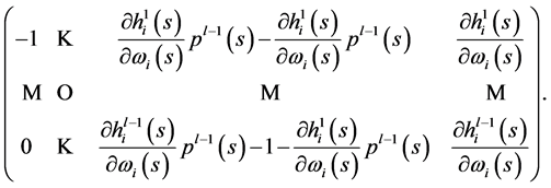
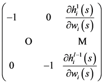
By simple algebraic manipulations we obtain the new matrices

Finally, we obtain

from which we extract the information required. Rank is equal to in every state. By the regular value theorem is a smooth manifold. This manifold is parameterized by smooth coordinate functions. From the regular value theorem it also follows that its dimension is equal to the dimension of minus, hence

.

The following theorem illustrates other economically interesting global properties of the equilibrium manifold. It says that by construction of a diffeomorphism restricted to the equilibrium manifold into

that is diffeomorphic to the sphere in implying that the equilibrium manifold is arc-connected, simply connected, and contractible. These properties are particularly useful in applied work such as economic policy equilibrium analysis.5 For example, economic policy is often concerned with finding a path between a current point on and a desired point on.

Theorem 4. The smooth equilibrium manifold of model is diffeomorphic to the sphere of dimension.

Proof. The aim of the proof is to define two smooth mappings between smooth manifolds such that we can apply the theorem (Hirsch [10] , pp. 15-16). Hence, let

be smooth mappings defined by

Then, let

denote smooth mappings defined by

Observe that the coordinates for the good of the m − 1 consumers in, are defined

(6)

Also observe that the coordinates for the consumer of the goods in, are defined by

(7)

The application of theorem ([10] ) requires to show that and that. The first part of the proof requires to calculate two inclusions, (i) and (ii). We start by showing the se- cond part first. Now, to show that (i), take any consumption bundle

,

and compute the inner product of (7) with , and apply Walras’ law to obtain

From that a reformulation of (7) readily follows in terms of the equilibrium equation

This is the equilibrium Equation (5), hence. Next, need to show that (ii). Take. It is then trivial to do the computations proving following equality

from which it readily follows that. Clearly we have constructed the two smooth relations such that

where is the identity map defined on. We have shown that the smooth mapping restricted to the equilibrium manifold defines a diffeomorphism between and the sphere of dimension.

It remains to be shown that equilibria in the long run production model with uncertainty always exist. The strategy of the proof is to show that the natural projection mapping is smooth and proper. Existence of long run equilibria of the production model with uncertainty follows immediately from the smoothness lemma (1) and the properness lemma (2) below.

Theorem 5. Equilibria of the two period production model with uncertainty always exist.

Lemma 1 (Smoothness) is smooth.

Proof. Recall that is a smooth submanifold of. It follows from the definition of a smooth manifold that its natural embedding is itself smooth. The projection mapping being itself smooth, it follows that the restriction of the natural projection to as the composition of two smooth mappings is therefore smooth.

The next lemma makes use of theorem (see [11] , p. 174).

Lemma 2 (Properness) is proper.

Proof. Pick an arbitrary for. Let be an element in a compact set. Now, for every and need to show (i) that is bounded from below. It follows that

and by non-satiation have also

which by monotonicity of implies that

Clearly, there exists some for every and satisfying

by boundedness of indifference mappings from below for every. (ii) We now show that for every and, is also bounded from above. For have

where

Clearly, , is bounded above by some, since for, is bounded from above for every. Hence have established upper and lower bounds defining a compact set

for every. Let G be a compact set defined by the preimage of the diffeomorphism projected onto. Now, by continuity of, is closed in, which by theorem (2) is a closed subset of. Closedness of follows from closedness of.

The number of equilibria of the long run production model with uncertainty is odd for any regular economy. The modulo 2 degree of is. See Guillemin and Pollack for example [12] .

I now define a subset of points on at which pairs are not regular.

Definition 2. is the set of singular equilibria given by the singular points of.

Proposition 1. is closed.

Proof. A necessary and sufficient condition for an equilibrium pair to be singular is that the determinant of the Jacobian matrix of, denoted by is equal to zero. Now, the set of critical points defined by the preimage of is closed by the closed mapping lemma ([9] ), since, , and the coefficients of, are all continuous, from which the result follows.

Definition 3..

A singular value is the image of of a singular point into. The set of regular values is defined by. It follows that represents the sets of regular economies. The next proposition states the is closed and of measure zero. This means that the probability of observing an economy with this property is “close” to zero. Hence, its complement is an open dense set.

Proposition 2. The set of singular economies is closed and of Lebesgue measure zero in.

Proof. The proof follows from the application of Sards’s theorem which describes the set of singular values of a smooth mapping having the property of Lebesgue measure zero. Hence know that is a set of Lebesgue measure zero. Closedness of follows from the properness of.

3. Conclusion

This paper discusses local and global equilibrium properties of a production economy with a long-term time structure. Production is modeled in the demand functions of the consumers. The advantage of this way of modeling production is that it enables us to establish a relationship between production and pure exchange economies. Adding uncertainty to the production model is a further step towards realism. It is shown that the equilibrium set of all production economies with uncertainty has the structure of a smooth submanifold of the Euclidean space which is diffeomorphic to a sphere. These topological properties are of significant economic importance in terms of economic policy design since they imply connectedness and contractability of the set of solutions. It is also shown that the set of singularities of the catastrophe map is closed, and of Lebesuge measure zero. The practical implication of this result is that the probability of observing an economy with a discontinuous price system is close to zero.

References

NOTES

¹Discussion paper: the natural projection approach to smooth production economies, 2011.

³“Smoothness” follows from the same reasons as in the previous section [8] . It essentially means that all functions are differentiable at any order required.

⁵The construction of a Riemanian metric on the equilibrium manifold would be a very useful result towards economic policy analysis.

References

- Debreu, G. (1959) Theory of Value. Wiley, New York.
- Arrow, K. and Debreu, G. (1954) Existence of an Equilibrium for a Competitive Economy. Econometrics, 22, 265-290. http://dx.doi.org/10.2307/1907353
- Balasko, Y. (1988) The Equilibrium Manifold: Postmodern Developments in the Theory of General Economic Equilibrium. The MIT Press, Cambridge, Massachusetts.
- Jouini, E. (1993) The Graph of the Walras Correspondence. The Production Economies Cas. Journal of Mathematical Economics, 22, 139-147. http://dx.doi.org/10.1016/0304-4068(93)90043-K
- Fuchs, G. (1974) Private Ownership Economies with a Finite Number of Equilibria. Journal of Mathematical Economics, 1, 141-158. http://dx.doi.org/10.1016/0304-4068(74)90005-6
- Stiefenhofer, P. (2011) Equilibrium Structure of Production Economies with Uncertainty: The Natural Projection Approach. Discussion Papers in Economics, University of York, York, 7.
- Stiefenhofer, P. (2013) The Catastrophe Map of a Two Period Production Model with Uncertainty. Applied Mathematics, 4, No. 8A.
- Debreu, G. (1972) Smooth Preferences. Econometrica, 40, 603-615. http://dx.doi.org/10.2307/1912956
- Lee, J.M. (2004) Introduction to Topological Manifolds. Springer, New York.
- Hirsch, M. (1972) Differential Topology. Springer Verlag, New York.
- Lee, J.M. (2000) Introduction to Smooth Manifolds. Springer, New York.
- Guillemin, V. and Pollack, A. (1974) Differential Topology. Prentice Hall, Upper Saddle River.
NOTES
1Discussion paper: the natural projection approach to smooth production economies, 2011.
3“Smoothness” follows from the same reasons as in the previous section [8] . It essentially means that all functions are differentiable at any order required.
5The construction of a Riemanian metric on the equilibrium manifold would be a very useful result towards economic policy analysis.