Received 20 March 2014; revised 20 April 2014; accepted 27 April 2014

ABSTRACT

A new modification of the Method of Lines is proposed for the solution of first order partial differential equations. The accuracy of the method is shown with the matrix analysis. The method is applied to a number of test problems, on uniform grids, to compare the accuracy and computational efficiency with the standard method.

Keywords:

Method of lines, first-order hyperbolic equation, numerical solution

1. Introduction

The method of lines (MOL) or differential quadrature is one of the few techniques for solving partial differential equations (PDEs), which can be used successfully using computers. In the Numerical Method of Lines (NMOL) the PDE to be solved is transformed into a system of ordinary differential equations (ODEs) by discretizing all the independent variables but one [1] .

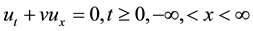
In this paper, first order hyperbolic partial differential equations depending on time and one spatial variable will be considered

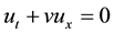(1)

In the case of equation (1) either t or x can be discretized, and the integration will be carried out along the remaining undiscretized independent variable.

The technique consists of converting the PDEs into ODEs either by finite difference spline, or by weighted- residual technique, then integrating the resulting ODEs [2] .

Finite differencing in the spatial variable led to a set of time dependent ODEs. The advantage of using MOL is that sophisticated software packages exist for the numerical solution of ordinary differential equations. These software packages contain iterative method for handling non-linearities and feature automatic step-size adjustment and integration order selection to maintain a specified error and to solve the problem with near optimal efficiency.

Several recently software packages for automated method of lines solution of arbitrarily defined PDEs have been very successful, particularly for parabolic and elliptic PDE systems.

We could improve the facilities for hyperbolic equations by incorporating an upwind weighted residual technique. This technique is similar to but superior to the use of an artificial viscosity term and could easily be used in any software package. Previous considerations of the MOL to solve PDEs have been geared to parabolic equation and generally used centered, second-order differences. Using these differences on hyperbolic equations can lead to unstable solution. To add stability, upstream (backward or forward) first-order differences could be used for the spatial discretization but these differences require the use of more grid points than central differences for a given spatial accord. An artificial dissipation (or viscosity) term is often added to a central differencing scheme to add stability but it is difficult to determine the magnitude of this term required for the stability and the effect of this term on the solutions.

Other stabilizing techniques that have been employed in the explicit finite difference procedures are generally not applicable to the method of lines approach because they involve manipulation of terms in both the time and space discretization.

In this paper, modified method of lines using a new three-point difference [3] is used.

Use of this new differences leads to stable schemes with good accuracy.

The method presented in this paper is attractive for hyperbolic, parabolic and elliptic partial differential equations.

2. Method of lines approximations

Consider the hyperbolic differential equation

With initial conditions

(2)

(3)

In order to apply the method of lines to equation (1), the spatial derivative must be approximated; an equally spaced mesh is used.

We might consider using finite differences scheme in the calculation of, as in Ref. [1] .

2.1. The centered difference

If we consider the centered difference scheme of order two

(4)

So

(5)

In this case, we observed that the centered differences produce excessive numerical oscillation in the solution to equation (1) because the eigenvalue of the system (5) is

which is pure imaginary so the system is unstable.

2.2. The upwind difference

One approach for improving the numerical solution is based partly on physical reasoning (since the flow is left to right or not), we might consider using upwind (or downwind) points in the calculation of. The simplest approximation that meets this requirement is the first order two-point upwind approximation.

(6)

These approximations eliminated the oscillation, but produced excessive numerical diffusion.

Therefore, we might again consider the upwind approximation, but with more grid point.

2.3. Good spatial discretization

As in the Ref. [3] we can use new difference scheme in the calculation of

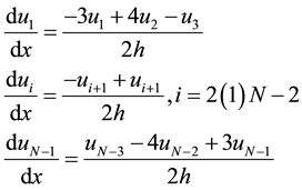(7)

which leads to stable schemes with good accuracy.

3. Analytical treatment of stability

There are two standard methods of the finite-difference equation. In the first, we express the equation in matrix form and examine the eigenvalues of the associated matrix; in the other method, we use a finite Fourier series. In this section we shall use the first method. The analysis of eigenvalues of the system gives necessary conditions for the stability of discretization of the problem [4] , which is should be real and negative values.

If we consider equation (1) with the discretization relation (5) then we get

where is

Mathematically the difference scheme is stable if there exists a real positive eigenvalues.

However, where is a tri-diagonal matrix, the corresponding eigenvalue of can be calculated from the relation.

where.

Thus

which are pure imaginary values.

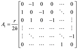
So, we consider the non-centered formula approximation

with the matrix formula

where

Thus the eigenvalues are given by

These values are real and negative, so the difference scheme is stable.

4. Numerical examples

In this section, some examples are considered to show the efficiency of the method.

4.1. Example (1)

Consider the following advection equation

With the conditions

With the analytic solution

In order to confirm the accuracy and efficiency of the method, the and error norms are used and defined by

where denote to the exact solution and denote to the numerical solution.

In the table 1 we examine various time step for the and error norms.

4.2. Example (2)

Consider the advection equation

With the condition

And the exact solution

In Table 2 show the and error norms.

4.3. Example (3)

Consider the equation

and

with the analytic solution

Table 3 produces the and for this problem.

5. Conclusions

In this paper, the modified method of lines is used to approximate the first order hyperbolic differential equation. Thus equations are one of the most difficult classes of PDEs to integrate numerically. To overcome this, we will suggest a modified MOL scheme.

The results are in good agreement with the exact solution as shown in Tables 1-3. The presented method is attractive for hyperbolic, parabolic and elliptic equations.

References

- Smith, G.D. (1985) Numerical Solution of Partial Differential Equations (Finite Difference Methods). 3rd Edition, Oxford University Press, Oxford.
- Schiesser, W.E. (1978) The Numerical Method of Lines: Integration of Partial Differential Equations. 2nd Edition, Clarendon Presses, Oxford.
- Sharaf, A.A. and Bakodah, H.O. (2005) A Good Spatial Discretization in the Method of Lines. Applied Mathematics and Computation, 171-172, 1253-1263.
- Carver, M.B. and Hinds, H.W. (1978) The Method of lines and the Advective Equation. Simulation, 31, 59-69.