Applied Mathematics
Vol.5 No.12(2014), Article
ID:47389,10
pages
DOI:10.4236/am.2014.512172
Mathematical and Physical Fractals
R. J. Slobodrian
Université Laval, Département de Physique, De Génie Physique et d’Optique, Québec, Canada
Email: rjslobod@phy.ulaval.ca, rjslobodrian@hotmail.com
Copyright © 2014 by author and Scientific Research Publishing Inc.
This work is licensed under the Creative Commons Attribution International License (CC BY).
http://creativecommons.org/licenses/by/4.0/


Received 15 February 2014; revised 19 March 2014; accepted 27 March 2014
ABSTRACT
A review of the concepts developed about mathematical and physical fractals is presented followed by experimental results of the latter, considered to be a fourth state of matter which pervades the universe from galaxies to submicroscopic systems. A model of multiple fractal aggregation via a computer code is shown to closely simulate physical fractals experiments carried out in simulated and in real low gravity.
Keywords:Fractal, Dimension, Aggregations, Evaporation-Condensation, Topology, Computer Simulations

1. Introduction
Fractal geometry and structures pervade our universe, living matter included. The field of fractals has developed after the advent of fast digital computers which provides easy means for their study. The word fractal was coined by Benoît Mandelbrot [1] , who also introduced the concepts of fractal geometry and fractal dimension. The foundations for the new developments were laid by 19th and 18th century mathematicians, particularly Cavalieri, Cantor, Lebesgue, Hausdorff, Besicovitch, Banach, Borel, Kuratowski and Kolmogorov, who developed the concepts of topological and metric spaces as well as a rigorous theory of measures, crucial to the understanding of the generalisation of the concept of dimension, leading to non-integer values (fractal dimensions).
Mandelbrot gave in 1982 a tentative definition of a fractal: A set for which the Hausdorff-Besicovitch dimension strictly exceeds the topological dimension. The latter are axiomatically 0 (zero) for a “point”, 1 (one) for a line, 2 (two) for a surface, etc. Mandelbrot retracted the definition given above because it would exclude many physical fractals and replace it introducing the concept of self-similarity: A fractal is a shape made by parts similar to the whole in some way [2] . This definition entails scale invariance of the appearance of parts of a whole. Physical fractals exhibit a finite range of scale where this invariance holds. Fractals in nature are mostly random structures showing disordered features. Fractal aggregates may be thought to be stochastic polymers and thus the smallest contituent discrete element is usually called monomer. Mathematical fractals are generated by algorithms (or a set of definite rules) and may exhibit an infinite range of scale invariance. They are sometimes called deterministic fractals.
1.1. A Mathematical Fractal
Work preceding the pleiade of recent developments includes examples justifying the introduction of the new concept of fractal dimension: one easy to grasp is the Cantor triadic dust [3] . The set is generated starting from a line segment C of unit length,
 (1)
(1)
and a sequence obtained by extracting successively the central third from each closed interval:
 (2)
(2)
 (3)
(3)
etc.
The sequence is shown in Figure 1 and is such that:
 (4)
(4)
Therefore Cantor’s set (Figure 1) can be expressed as follows
 (5)
(5)
It is a set with an infinite number of segments, a non dense subset of he original line segment converging to an infinite set of points: “dust” particles. The generic term of C consists of 2k closed intervals of length (1/3)k. Thus the total length of Ck is:
 (6)
(6)
and
 (7)
(7)
Therefore, although the Cantor “dust” contains an infinite subset of points of [0,1] distributed along the segment it is of topological dimension 0 as shown. Such dimension corresponds to a single point and logically it should be expected that an infinite set of points should be reflected by a more meaningful parameter than that of topological dimensions. It is necessary to remember how we usually “measure” bodies, surfaces or lines. For example, considering the floor in a room it is possible to use surface elements of variable linear dimension e to cover the set to any desired accuracy. The “capacity” CA of a covering element can be expressed in general as
 (8)
(8)
For squares K = 1, for disks K = p, with n = 2, for spheres K = 4/3p, n = 3.
The area A of a floor can be given by a covering with N elements as
 (9)
(9)
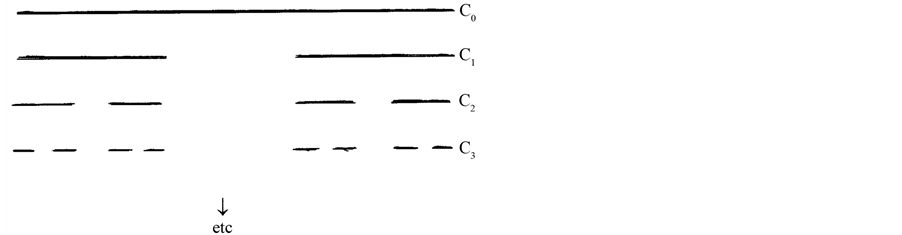
Figure 1. Cantor’s triadic dust.
If the surface to be measured is not dense, (like the one dimensional Cantor’s “dust”), it is possible to write formally a covering element as
 (10)
(10)
understandably  and it would account for the non-dense caracter of the surface, substituting the topological dimension of a surface. Choosing A = 1 the following expression is obtained:
 (11)
(11)
 (12)
(12)
Taking the limit the term in K can be omitted and then one obtains a definition for the fractal dimension D:
 (13)
(13)
This definition follows closely those of Kolmogorov (1958) [4] and of Mandelbrot (1982) The symbol 1 represents the set and e is the linear dimension of the element to cover it, the latter is often called “ball”. Assume now that 1 is the segment [0,1]. Evidently , and therefore expression (13) yields D = 1, coincident with the topological dimension of a solid line. Applying this to Cantor’s triadic set (“dust”),
  and
and  and therefore
 (14)
(14)
And as surmised before the dimension D is non integer. A non dense set is thus reflected by a generalized dimension D fractal dimension exceeding the topological dimension.
1.2. Example of a Two Dimensional Fractal
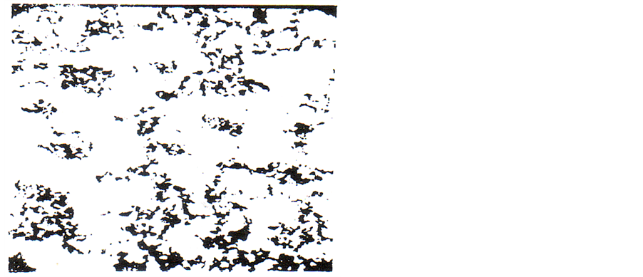
A two dimensional set of carbon particles (Figure 2(a)) demonstrates an application of preceding formulae. The experiment was carried out by deposition of the particles on a plate, after traversing a tetrachloride carbon liquid. The high density of the fluid allowed a slow random fall of the particles. The pattern was analyzed using a frame grabber system to construct Figure 2(b), where the slope yields the fractal dimension of the set.
 (a)
(a)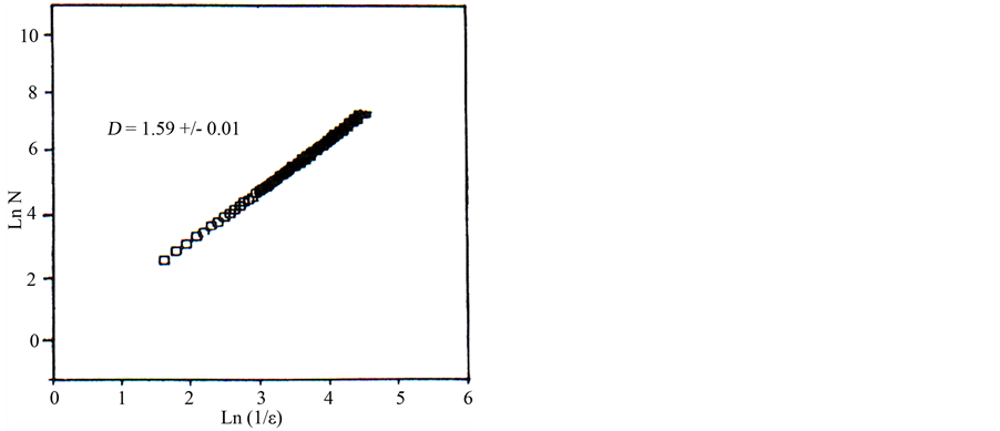 (b)
(b)
Figure 2. (a) 2-dimensional fractal; (b) a graph of its fractal dimension given by the slope of the line of points.
2. Physical Fractal Aggregates
In order to appeal to everyday life intuition let us mention snowflakes in free fall. They are the result of aggregation of water crystals during their fall through the atmosphere. Usually their velocity is constant due to aerodynamics. It simulates the behavior of aggregation of matter in a gravitation free environment. The latter has become available during the 20th century via aircraft in parabolic fight, and on space stations (Mir and ISS). Dust is ubiquitous in the Earth’s atmosphere and undergoes processes of aggregation leading to increased masses and precipitations on the earth’s surface. Cosmic dust pervades outer space and the study of its behavior is now possible. Flotation is also a means to simulate conditions of reduced gravity. Flotation in water is used for training of astronauts. Flotation of small particles in gases also allows studying aggregation processes simulating low gravity.
2.1. Nomenclature of Fractals
A typical fractal aggregate is shown in Figure 3. Self similarity and scale invariance is demonstrated by the small aggregate on the upper right side. The constituent particles are spherical but fractals may be formed by units of varied forms (v.l. micro-crystals).
2.2. Computer Simulation of Aggregation
The physical process is random and this characteristic should provide the mathematical basis for simulations of aggregation. Figure 4 shows a computer generated aggregate. The constituent particles are spherical and radii
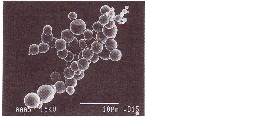
Figure 3. Scanning electron microscope (SEM) image of a 3D aggregate. The procedure of production is described in [7] .
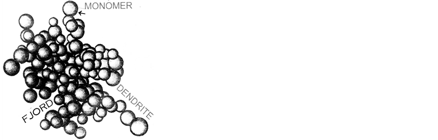
Figure 4. Computer simulated aggregate.
are variable, the usual name is monomer by analogy with chemical polymers. Branches are called dendrites (from Greek: dendros: tree). The deep valleys are called fjords (from Norwegian: inlet). The computer program consists of sections: 1) Generation of aggregates via random walk paths and attachment of monomers; 2) Graphical display of the result; 3) Printing of the graph.
This image is shown with shadows as illuminated by a light slightly skewed from the left. Multiple fractal aggregation shall be discussed further down in this paper.
2.3. Low Gravity Powder Aggregates
They were carried out on aircraft in parabolic flight and also on the space shuttle. Figure 5 shows the schematic of an apparatus flown on NASA’s KC-135 aircraft. It allows the simultaneous recording of two perpendicular images of the experimental volume via an optical system with a prism. This technique allows a perfect synchronization of the images. This is the experimental recoding of images in the Monge geometrical projections. Figure 6(a) and Figure 6(b) shows images of aggregates obtained.
Blum et al. [6] carried out experiments on particle aggregation on the Space Shutttle. The main results are shown below in Figure 7.
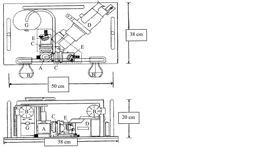
Figure 5. Powder aggregation apparatus [5] . A. Experimental cell; B: Bellows; C. Lens assembly; D. Camera; E. Mirrors; F. Prism.
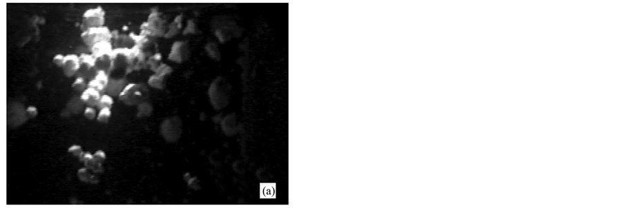
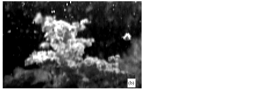
Figure 6. (a) & (b) Powder aggregates images recorded in parabolic flight.
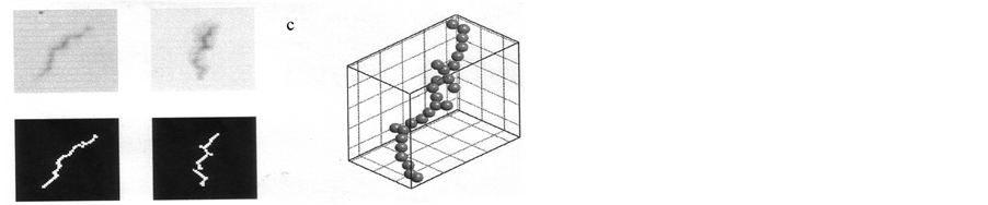
The top images are the raw data, below are reconstructed images, at right is a three dimensional image from the lower images, proving aggregation and also the formation of proto planets from cosmic dust via such process.
3. Evaporation—Condensation Aggregation
Condensation of matter in vapor form yields aggregates at variance with powder aggregations. The latter are due to surface adherence of monomers and there is no matter continuity throughout the aggregate. The former result in topological connected sets of monomers as is illustrated in Figure 8. They are synterized [7] . Figure 9 shows the full aggregate.
Aggregates with typical monomers were analyzed by scattering of He-Ne laser radiation (Figure 10) to determine the fractal dimension D from the angular distribution of the intensity I(q), where q is the modulus of the initial to final wave vectors (Figure 11). This is a non-destructive indirect measurement method.
4. Multiple Fractal Aggregations and Simulations
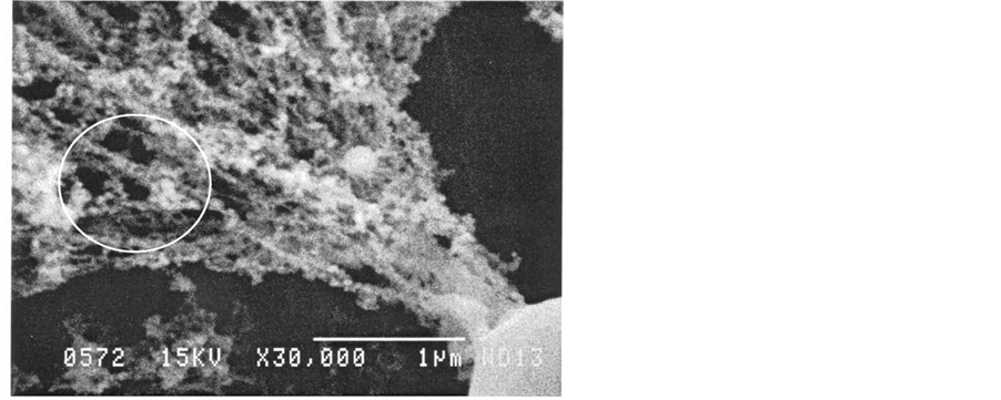
Aggregations take place at random in the available volume and multiple aggregates are formed. Figure 12 illustrates the complexity of aggregates generated simultaneously. Simulation of multiple aggregations are shown in Figure 13 with our program. Similarly Figure 14(a) shows an inset which is adequately simulated.
5. Concluding Remarks: Fractal Physics
Classical physics is based on fundamental continuity of space and time. Quantum phenomena have introduced discontinuity concepts (“jumps”) in physics, but they are interpreted in terms of equations within continuous space and time. There are fundamental questions concerning the transition between quantized and classical realms but they are not yet resolved. On occasion so called semiclassical physics can be applied successfully to phenomena [8] but doubts have been raised repeatedly about the validity of the correspondence principle of Niels Bohr [9] . It has been recently recognized that certain phenomena within this transition region can be classified in a new domain: fractal physics [10] , with special topological content, discrete entities and intrinsic randomness. Most importantly it has been realized that fractal physics pervades the whole universe at all scales in space and time.
The aggregates obtained correspond to an underlying randomness and provide examples of complexity in dynamical systems [11] . The sizes of monomers obtained imply that they are within the realm of the transition region from quantum to classical phenomena and they may provide a testing ground for the validity of Bohr’s correspondence principle. The nanometer scale yields matter where surfaces are extremely large with respect to the volume. The ratio is increased by a factor of 107 as compared with the ratio for ordinary compact matter at cm scales. These aggregates are certainly manifestations of a new state of matter [12] , and bear promise of novel physical properties and applications.
Acknowledgements
Space agencies of Canada, Europe and USA have supported the research of this paper over many years and they are warmly thanked. The program FRAC was written by Drs. Eric Litvak and Carl Robert, they are thanked heartily.
My colleagues Drs. Claude Rioux and Michel Piché have contributed with experimental instruments, exper-
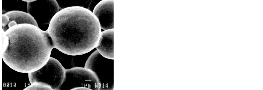
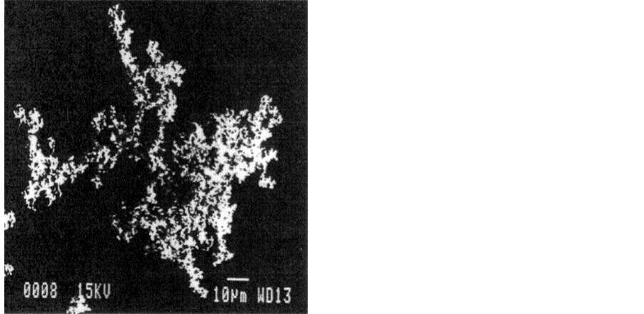
Figure 9. Zn aggregate via vapor condensation.
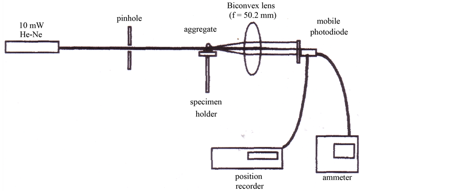
Figure 10. Set-up to measure a fractal dimension by scattering of a laser beam. It is a non destructive method.
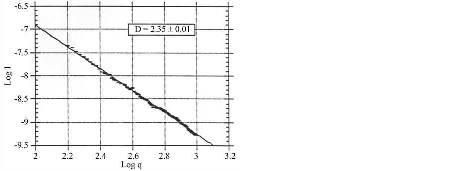
Figure 11. Example of a measurement with the set-up of Figure 10. The line (straight) proves fractality and its slope gives a measure of its dimension.
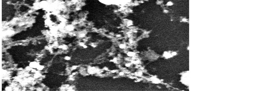
Figure 12. Experimental multiple aggregation.
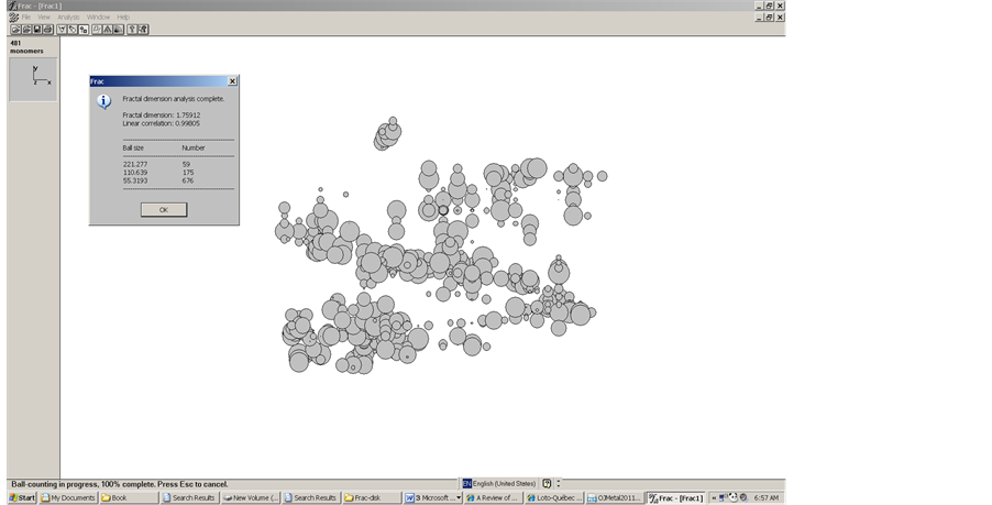
Figure 13. Simulation of multiple aggregation with our program 3DMXYF, the graph was obtained with program FRAC which calculated its fractal dimension.
 (a)
(a)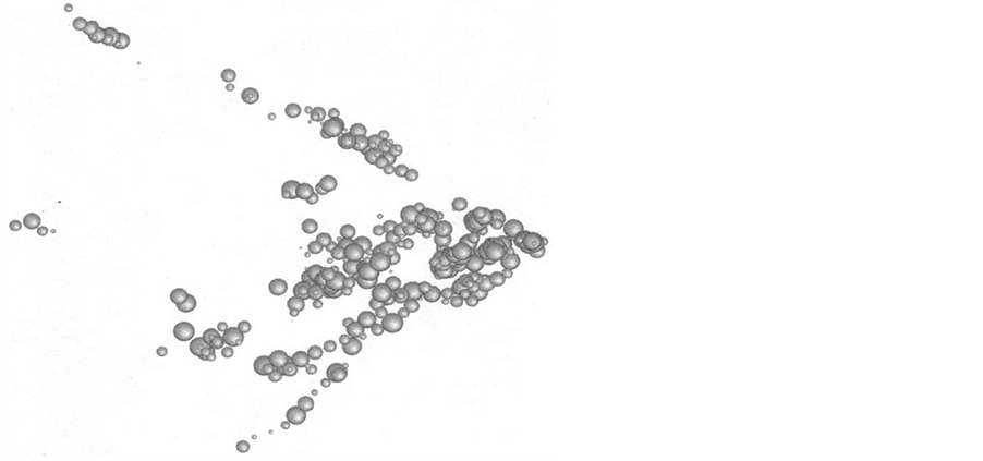 (b)
(b)
Figure 14. (a) SEM image of an aggregate; (b) Multiple aggregation simulation. Notice the similarity with (a) in the circle.
tise and laser set ups for the study of physical fractals and are kindly thanked. The team of the SEM has provided excellent images of fractal aggregates and deserve warmest thanks.
References
- Mandelbrot, B. (1982) The Fractal Geometry of Nature. Freeman, San Francisco.
- Mandelbrot, B. (1989) Les Objets Fractals, Forme, Hasard, Dimension. 3rd Edition, Flammarion, Paris.
- Cantor, G. (1883) über unendliche, lineare Punktmannigfaltigkeiten V. Mathematische Annalen, 21, 545-591. http://dx.doi.org/10.1007/BF01446819
- Kolmogorov, A.N. and Tihomirov, V.M. (1993) Classics on Fractals. Addison-Wesley Pub. Co., Boston.
- Rioux, C., Potvin, L. and Slobodrian, R.J. (1995) Particle-Particle Aggregation with 1/r2 Forces in Reduced Gravity Environments. Physical Review, E52, 2099. http://dx.doi.org/10.1103/PhysRevE.52.2099
- Blum, J., et al. (2000) Growth and Form of Planetary Seedlings: Results from a Microgravity Aggregation Experiment. Physical Review Letters, 85, 2426.
- Slobodrian, R.J. (2013) Metallic Fractal Aggregates and Monomers. LAP LAMBERT, Saabrücken.
- Brack, M. and Bhaduri, R.K. (1997) Semiclassical Physics. Addison Wesley, Boston.
- Bohr, N. (1923) über die Anwendung der Quantentheorie auf den Atombau. Zeitschrift für Physik, 13, 117-165. http://dx.doi.org/10.1007/BF01328209
- Pietronero, L. (Ed.) (1989) Fractals’ Physical Origin an Properties. Plenum Press, New York. http://dx.doi.org/10.1007/978-1-4899-3499-4
- Grassberger, P. (1990) Information and Complexity Measures in Dynamical Systems. Plenum Press, New York.
- Task Group on Fundamental Physics and Chemistry (1988) Space Science in the Twenty First Century: Imperatives for the Decades 1995 to 2015. National Academy Press, Washington D.C.