Applied Mathematics
Vol.5 No.2(2014), Article ID:42170,8 pages DOI:10.4236/am.2014.52030
The Optimal Inventory Policy for Reusable Items with Random Planning Horizon Considering Present Value
1Department of Banking and Finance, Takming University of Science and Technology, Taiwan
2Department of Applied Mathematics and Business Administration, Chung Yuan Christian University, Taiwan
3Department of Applied Mathematics, Chung Yuan Christian University, Taiwan
Email: meimei@takming.edu.tw, *shyder@cycu.edu.tw, shau.tang@msa.hinet.net
Received November 11, 2013; revised December 11, 2013; accepted December 19, 2013
ABSTRACT
We discuss five areas of inventory model, including reusable raw material, EPQ model, optimization, random planning horizon and present value. In the traditional EPQ model, the stock-holding cost of raw material was not counted as a part of relevant cost. We explored the possibility of reducing a company’s impact on the environment and increasing their competitiveness by recycling their repair and waste disposal. The products are manufactured with reusable raw material. Our analysis takes into account the time value, and the present value method is applied to determine the optimal inventory policies for reusable items with random planning horizon. Results show how the heuristic approach can achieve global optimum. Numerical examples are given to validate the proposed system.
Keywords:Reusable; EPQ; Optimization; Random Planning Horizon; Present Value
1. Introduction
Reuse of material and products is not a new subject. Using the repaired and new made products, Richter [1] has created a model for fixed and variable collection time interval to minimize the cost and found the optimal collection intervals. Richter and Dobos [2] extended the model of Richter [3] with integer setup numbers. By applying Pontryagin’s Maximum Principle, Kleber et al. [4] determined the optional production, remanufacturing, and disposal policy for a cost model. Koh et al. [5] found a joint EOQ and EPQ model in which a fixed proportion of the used products is collected from customers and then recovered for reuse. Konstantaras and Papachristos [6] revised Koh et al.’s paper and used a different analysis to obtain closed form expressions for both the optimal number of setup in the recovery and the ordering processes. Karakayal et al. [7] characterized the optimal acquisition price of the used products and the selling price along with recovery quantities of the reusable components. Up to now Salameh & El-Kassar [8] had the paper to establish an EPQ model taking the stock-holding cost of raw material into consideration and found the optimal lot size. El-Kassaret et al. [9] studied an EPQ model for imperfect quality raw material.
The EOQ (Economic Ordering Quantity) model was first proposed by Harris [10] and later the EPQ model was developed by E. W. Taft [11]. This paper is mainly based on Richter’s ([1,3]) and Moon and Yun’s [12] idea, and followed the research of Trippi [13], Kim, Philippatos and Chung [14], Moon and Yun [12] and Chung and Lin [15] about time value of money. Kim, Philippatos and Chung [14] have showed a method for evaluating investments in inventory. Moon and Yun [12] have justified the optimality of solutions which are derived from the first order conditions in Kim, Philippatos and Chung [14]. Later Chung and Lin [15] have derived the bounds for the optimal cycle following the optimality of solutions. Using the upper and lower bounds, an algorithm of computing the optimal cycle time is developed. These numerical examples are brought into the algorithm to find the different cycle time. We wish this model is appropriate and practical.
2. The Models
The mathematical models developed in this study are based on the following definitions and assumptions.
Definitions:
PVC(T): the present value of the cash flow for the first inventory horizonC(T): the expected present value of the cash flow for the random planning horizonTRC(T): the total relevant cost per unit timeQ: the order sizeS: the cost of placing an orderP: the production rateD: the demand rateC: the purchasing cost per unit item,
 : the reusable rateT: the cycle lengthr: the discount rateh: the stock holding cost of raw materials per item per year and the stock holding cost of finished products per item per yearx: the random planning horizon time.
Assumptions:
1) Production rate is greater than demand rate.
2) Production rate and demand rate are known and constant.
3) Shortage is not allowed.
4) A single item is considered.
5) The time horizon is not infinite.
6) The stock holding cost of raw materials and products are the same.
7)![]() .
.
8) At the end of the planning horizon, the raw material is used up and the productions are sold out.
9) The random planning horizon time x follows an exponential distribution with parameter![]() .
.
Two models used in this analysis are illustrated below (see Figure 1). Model 1 presents the annual total relevant cost, TRC(T). Model 2 presents the expected present value of total relevant cost for the random planning horizon, C(T). The analysis proceeds as follows. First, we find the optimal cycle time separately for each model. Then, we use the numerical examples to show how to find the optimal value of cycle time.
Model 1: We use the annual total relevant cost to find the optimal solution.
The annual total relevant cost TRC(T) consists of the following elements:
The ordering cost per unit time =![]() .
.
The purchasing cost per order per unit time = .
.
The stock holding cost of raw material per unit time = .
.
The stock holding cost of products per unit time = .
.

Figure 1. Raw material inventory level and products inventory level.
The total relevant cost per unit time can be expressed as TRC(T) = the ordering cost per unit time
+ the purchasing cost per order per unit time
+ the stock holding cost of raw material per unit time
+ the stock holding cost of products per unit time
= 
The first and second derivatives of TRC(T) are
 and
and  for all T > 0, respectively.
Set , then we have the following result:

The unique solution of above equation is 
At , the TRC(T) has a global minimum on (0,
![]() ) since
) since  for all T > 0.
Model 2: Using the expected present value of total relevant cost for random planning horizon C(T) to find the optimal solution.
We assume that the random planning horizon x is located on the (k + 1)th cycle time. The present value of total relevant cost at the first cycle time PVC(T) consists of the following elements:
The ordering cost = S.
The purchasing cost = .
.
The stock holding cost of raw material = .
.
The stock holding cost of products = .
.
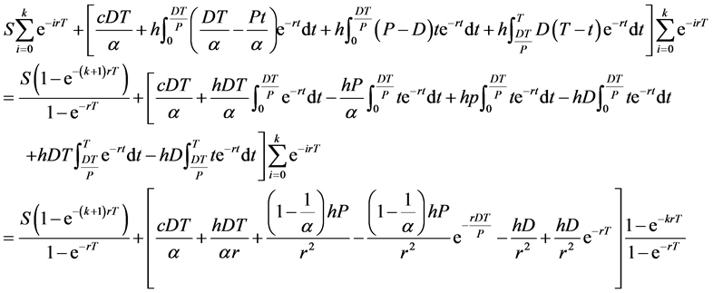
The present value of total relevant cost at the first cycle time PVC(T) is as follows:
 .
.
The present value of total relevant cost from the beginning of the first cycle time to the beginning of the (k + 1)th cycle time is as follows:
 (1)
(1)
The present value (at time of kT) of total relevant cost at the (k + 1)th cycle time consists of the following elements:
The purchasing cost = .
.
The stock holding cost of raw material = .
.
The stock holding cost of products = .
.
The present value of total relevant cost at the (k + 1)th cycle time is as follows:
 (2)
(2)
Now, we want to find the expected present value of total relevant cost for random planning horizon C(T).
The present value of total relevant cost includes:
(A) The present value of total relevant cost from the beginning of the first cycle time to the beginning of the (k+1)th cycle time.
(B) The present value of total relevant cost at the (k + 1)th cycle time.
If we assume that the probability density function of x is![]() , the expected present value of the total relevant cost from the beginning to the time x is C(T).
, the expected present value of the total relevant cost from the beginning to the time x is C(T).
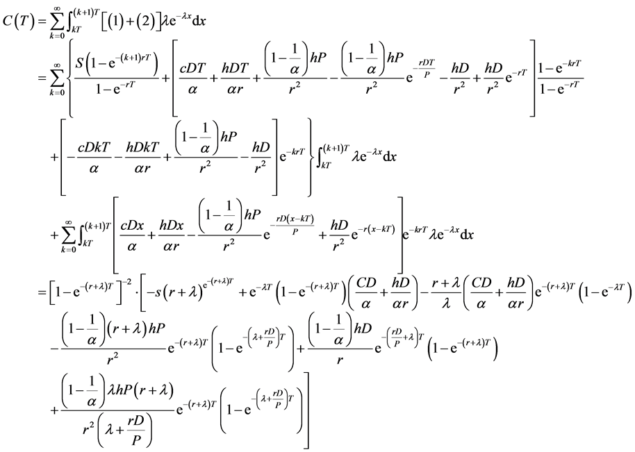 (3)
(3)
Let 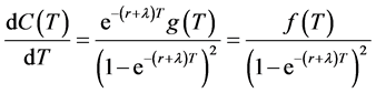 (4)
(4)
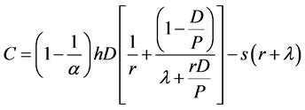
where
 . (5)
. (5)
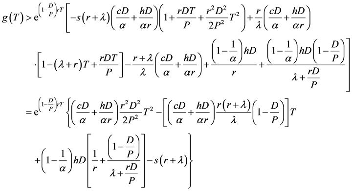
Then we obtain the first derivative of g(T) as follows:
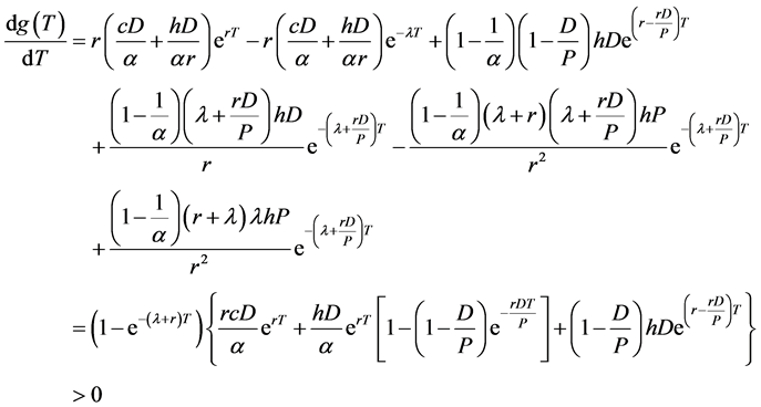 (6)
(6)
Since  and
and , the equation
  has a unique solution.
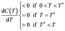
From the calculations described above, we have proved that . Thus,
  is a strictly increasing function. From the results above, we conclude that
  has a unique solution
  as shown in the following:
 . (7)
. (7)
Since , it is therefore implied that there is a unique solution
  as shown in the following:
 . (8)
. (8)
It is not easy to solve  out in this case. Our first step is to find an upper and an lower bound of
 . Then, we used the Intermediate Value Theorem and the algorithm of bisection method to find the optimal cycle time. We will now show the procedure of finding a lower bound
  and an upper bound
 .
.
We set the lower bound as , and then we found an upper bound of
 :
:
 . (9)
. (9)
Setting
 , (10)
 , (11)
 . (12)
And from the above, we can now simplify the inequality to
 , (13)
The positive solution of  is
is
 (14)
(14)
Theorem: 
Proof: Since  is a strictly increasing function, we conclude that
 ![]() for all T and
for all T and .
.
By Equation (97),
 (15)
(15)
 (16)
(16)
 (17)
(17)
From the above, (18)
(18)
Now we can compute the exact optimal cycle length  of model 2 by using the logic of the following algorithm. Our method is similar to the one of Chung and Lin (see [15]).
Step 1: Let ![]()
Step 2: Set  and
and 
where ,
,

 .
.
Step 3: Set 
Step 4: If , go to Step 6.
Otherwise go to Step 5.
Step 5: If , then we set
![]() .
.
And if , then we set
![]() .
.
Then go to Step 3.
Step 6:![]() Where
Where  is the optimal cycle length.
3. Numerical Examples
Example 1: If we set the numbers as S = 1000, P = 2000, D = 1500, c = 10, ![]() ,
, ![]() , r = 0.15, h = 2 and
, r = 0.15, h = 2 and![]() , then we have
, then we have  and
and .
.
Example 2: If we set the numbers as S = 2000, P = 2000, D = 1500, c = 10, ![]() ,
, ![]() , r = 0.15, h = 2 and
, r = 0.15, h = 2 and![]() , then we have
, then we have  and
and .
.
Example 3: If we set the numbers as S = 1000, P = 2000, D = 1500, c = 20, ![]() ,
, ![]() , r = 0.15, h = 2 and
, r = 0.15, h = 2 and![]() , then we have
, then we have  and
and .
.
Example 4: If we set the numbers as S = 1000, P = 2000, D = 1500, c = 10, ![]() ,
, ![]() , r = 0.15, h = 2 and
, r = 0.15, h = 2 and![]() , then we have
, then we have  and
and .
.
Example 5: If we set the numbers as S = 1000, P = 2000, D = 1500, c = 10, ![]() ,
, ![]() , r = 0.1, h = 2 and
, r = 0.1, h = 2 and![]() , then we have
, then we have  and
and .
.
Example 6: If we set the numbers as S = 1000, P = 2000, D = 1500, c = 10, ![]() ,
, ![]() , r = 0.15, h = 2 and
, r = 0.15, h = 2 and![]() , then we have
, then we have  and
and .
.
4. Conclusion
The planning horizon is random and has an exponential distribution with a parameter that influences the optimal cycle time. The raw material is used up and the products are sold out at the end of the planning horizon. Thus, the results are more economical in this model. The use of reusable raw material is beneficial and worthwhile. The models in this research can be applied in companies that use reusable or new raw material. There are many interesting results derived from the numerical examples that future research should take into consideration. It is not necessary for the stocking holding cost of raw material and the stock holding cost of products to be the same.
REFERENCES
- K. Richter, “The Extended EOQ Repair and Wasted Disposal Model with Variable Setup Number,” European Journal of Operational Research, Vol. 96, No. 2, 1996, pp. 313-324. http://dx.doi.org/10.1016/0377-2217(95)00276-6
- K. Richter and I. Dobos, “Analysis of the EOQ Repair and Waste Disposal Problem with Integer Setup Numbers,” International Journal of Production Economics, Vol. 45, No. 1-3, 1999, pp. 443-447. http://dx.doi.org/10.1016/0925-5273(95)00143-3
- K. Richter, “The Extended EOQ Repair and Wasted Disposal Model,” International Journal of Production Economics, Vol. 59, No. 1-3, 1996, pp. 463-467. http://dx.doi.org/10.1016/S0925-5273(98)00110-8
- R. Kleber, S. Ninner and G. P. Kies Muller, “A Continuous Time Inventory Model for a Product Recovery System with Multiple Options,” International Journal of Production Economics, Vol. 79, No. 2, 2002, pp. 121-141. http://dx.doi.org/10.1016/S0925-5273(02)00256-6
- S. G. Koh, H. Hwang and C. S. Ko, “An Optimal Ordering and Recovery Policy for Reusable Items,” Computers and Industrial Engineering, Vol. 43, No. 1-2, 2002, pp. 59-73. http://dx.doi.org/10.1016/S0360-8352(02)00062-1
- I. Konstantaras and S. Papachristos, “Note on: An Optimal Ordering and Recovery Policy for Reusable Items,” Computers and Industrial Engineering, Vol. 55, No. 3, 2008, pp. 729-734. http://dx.doi.org/10.1016/j.cie.2008.02.007
- I. Karakayali, H. Emir-Farinas and E. Akcali, “Pricing and Recovery Planning for Demanufacturing Operations with Multiple Used Products and Multiple Reusable Components,” Computers and Industrial Engineering, Vol. 59, No. 1, 2010, pp. 55-63. http://dx.doi.org/10.1016/j.cie.2010.02.016
- M. K. Salameh and A. N. El-Kassar, “Accounting for the Holding Cost of Raw Material in the Production Model,” Proceeding of BIMA Inaugural Conference, Sharjah, 17-18 March 2007, pp. 72-81.
- A. N. El-Kassar, M. Salameh and M. Bitar, “EPQ Model with Imperfect Quality Raw Material,” Mathematica Balkanica, Vol. 26, 2012, pp. 123-132.
- F. W. Harris, “What Quantity to Make at Once,” The Library of Factory Management, Operation and Costs, A. W. Shaw Company, Chicago, Vol. V, 1915, pp. 47-36.
- E. W. Taft, “The Most Economical Production Lot,” The Iron Age, Vol. 101, May 30 1918, pp. 1410-1412.
- I. Moon and W. Yun, “An Economic Order Quantity Model with a Random Planning Horizon,” The Engineering Economist, Vol. 39, No. 1, 1993, pp. 77-86. http://dx.doi.org/10.1080/00137919308903113
- R. R. Trippi and D. E. Lewin, “A Present Value Formulation of the Classical EOQ Problem,” Decision Sciences, Vol. 5, No. 1, 1974, pp. 30-35. http://dx.doi.org/10.1111/j.1540-5915.1974.tb00592.x
- Y. H. Kim, C. C. Philippatos and K. H. Chung, “Evaluating Investments in Inventory Systems: A Net Present Value Framework,” The Engineering Economist, Vol. 31, No. 2, 1986, pp. 119-136. http://dx.doi.org/10.1080/00137918608902931
- K. J. Chung and S.-D. Lin, “A Note on the Optimal Cycle Length with a Random Planning Horizon,” The Engineering Economist, Vol. 40, No. 4, 1995, pp. 385-392. http://dx.doi.org/10.1080/00137919508903162
NOTES

*Corresponding author.