ABSTRACT

Our main aim is to prove a more general version of the quantum Zeno effect. Then we discuss some examples of the quantum Zeno effect. Furthermore, we discuss a possibility that based on the quantum Zeno effect and certain experiments one could check whether, from the statistical point of view, a concrete system behaves like a quantum system. The more general version of quantum Zeno effect can be helpful to prove that the brain acts like in a quantum system. The proof of our main result is based on certain formulas describing probability distributions of time series related to quantum measurements.

1. Introduction

Zeno of Elea (ca. 490 BC-ca. 430 BC) was one of the oldest Greek philosopher. Aristotle called him the inventor of the dialectic. He is best known for his paradoxes. The most famous are the so called “arguments against motion” described by Aristotle in his Physics. Let us mention Zeno’s arrow paradox which states that, since an arrow in flight is not seen to move during any single instant, it cannot possibly be moving at all. What does it mean? Let be the position of arrowhead at time. Then the arrow will move. denotes the position of the arrowhead at time. Now, let be a sequence of times. Then the observed positions of the arrowhead are represented by the sequence. If the distance of times is very small then the distance of the corresponding positions is very small. According to Zeno that implies that the arrow cannot move under continuous observation. Of course we know that this is nonsense because in classical mechanics observations are of no effect on the state of the system—not so in quantum mechanics where observation, i.e., measurement, causes a change of the state. That is the basic idea of the quantum Zeno effect.

The quantum Zeno effect is a name coined by George Sudarshan and Baidyanath Mirsa of the University of Texas in 1977 in their analysis of the situation in which an unstable particle, if observed continuously, will never decay [1]. One can “freeze” the evolution of the system by measuring it frequently enough in its (known) initial state. The meaning of the term has since expanded, leading to a more technical definition in which the time evolution can be suppressed not only by measurement [2,3]. That does not mean that there exists a complete theory of the quantum Zeno effect. Even there is no precise meaning concerning the notion of “suppression of the time evolution”.

An earlier theoretical exploration of this effect of measurement was published in 1974 by Degasperis et al. [4] and A. Turing described it in 1954 [5]: It is easy to show (but there was no rigorous proof!) using standard theory that if a system starts in an eigenstate of some observable, and measurements are made of that observable times a second, then even if the state is not a stationary one, the probability that system will be in the same state after, say, one second, tends to one as tends to infinity; that is, that continual observations will prevent motion.

The idea is contained in the early work by J. von Neumann, sometimes called the reduction postulate [6]. According to the reduction postulate, each measurement causes the wave function to “collapse” to a pure eigenstate of the measurement basis.

Usually the model of Turing is far from the reality, because in reality the state of the quantum system is usually unknown, and it is a mixed state. Furthermore that kind of measurements is not realistic, i.e., real measuring instruments cannot perform such kind of measurements. Nevertheless a general theory of the quantum Zeno effect should contain the Turing model as a special case.

Following A. Turing the reduction of the states seems to be the background of the quantum Zeno effect. Now our work on the quantum Zeno effect was motivated by the quantum model of certain brain activities developed in [7-15]. For that reason let us briefly mention what kind of reduction of states were considered in certain quantum models of brain activities.

In Wikipedia, the free encyclopedia on the Zeno effect is written the following:

1.1. Significance to Cognitive Science

The quantum Zeno effect is becoming a central concept in exploration of controversial theories of quantum mind consciousness within the discipline of cognitive science. In his book Mindful Universe (2007) (see also [16]), Henry Stapp claims that the mind holds the brain in a superposition of states using the quantum Zeno effect.

Now, let us consider the process of recognition of signals in the brain. Then the basic idea of Stapp may be described as follows: If there will be a signal arising from the senses, the process of recognition starts. That process represents a rapid sequence of “trials” checking whether the signal from the senses and the signal created by the brain partially coincide. He identifies these trials with measurements performed by a mysterious “observer” in the brain. That does not seem to be realistic.

Related to the model of recognition discussed in [7-15], these trials are not represented by a process of measurements. Nevertheless the results of the trials are represented by projections like in the case of measurements.

That R. Penrose [17,18] explains as follows: The conventional quantum theory view is that the quantum state reduces by measurement or observation (subjective reduction). Now, a number of physicists have argued in support of special models in which the rules of standard quantum mechanics are modified by the inclusion of some additional procedure according to which the reduction of the state becomes an objectively real process (objective reduction)—the system abruptly self-collapses. Consciousness, it is argued, requires non-computability. The only readily available apparent source of non-computability is self-collapse. The self-collapse, irreversible in time, creates an instantaneous “now” event. Sequences of such events create a flow of time, and consciousness.

That means recognition of signals is a process of self-collapses. That coincides with the basic idea of the quantum model of recognition of signals in the brain in [7-15]. Furthermore, like sequences of measurements that process suppresses a certain unitary time evolution in the brain. A lot of experiments show that there is a suppression of a certain process in the brain caused by the recognition of signals or some other kind of activities of the brain (cf. [19]).

Using series of measurements at different times one tries to get information on the statistical behaviour of certain random processes. That series of measurements give a so called time series.

1.2. Time Series—Classical Probability Theory

In classical stochastics one identifies the time evolution of a random system with a stochastic process taking on values in a certain space. The random variable represents the system at time. A measurement at a certain time one identifies with a certain (measurable) real function on, and the random number represents the output of the measurement.

Now, let us consider a sequence of time . At time one performs a measurement related to a function on. Then the sequence represents a so called time series.

If we would know the distribution of the underlying stochastic process, then we can calculate the distribution of the time series.

Sometimes specialists use the notion “time series” only in the special case:

.

That means one performs always the same measurements at equidistant times.

In order to obtain information concerning the state of the brain and its time evolution one has to perform several EEG measurements at different times. That gives a time series. In practice specialists use certain statistical methods evaluating that time series, i.e., they analyze the outcomes of the sequence of measurements. To make these statistical investigations effective, and precise from mathematical point of view one should know the type of the distribution of the stochastic process on the space of point configurations representing the time evolution of the configuration of excited neurons in the brain. Up to now that information is lacking (cf. [20]).

1.3. The Quantum Case of Time Series

Let be a semigroup of unitary operators on a separable Hilbert space representing the time evolution of a quantum system. denotes the state of the quantum system at time. We consider again a sequence of time and perform measurements at time related to selfadjoint operators given by their unique representation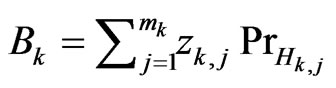, i.e., represents an orthogonal decomposition of and if. Because each realistic measuring instrument has a finite scale we consider only selfadjoint operators being of this type.

Formally we can identify the random outputs of these measurements with random numbers representing the time series in the considered quantum case.

Unfortunately, in the quantum case there does not exist a stochastic process such that we can always represent the distribution of the time series as follows:

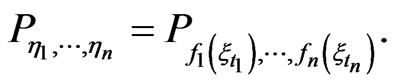
For that reason one has to develop a useful concept in order to describe the distribution of such time series related to quantum measurements. That will be done in Section 2 of this paper.

1.4. On the Quantum Zeno Effect

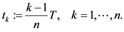
Starting with the notations used above we will specialize

That means we consider repeated measurements in the time interval according to starting at time with equidistant times. Again denotes the state of the quantum system at time, and the random numbers represent the outputs of the measurements.

In Section 3 of this paper we will prove the following theorem.

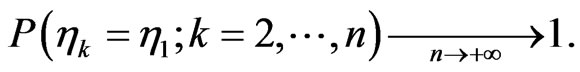
Theorem It holds

Immediately from the theorem we obtain the following corollary.

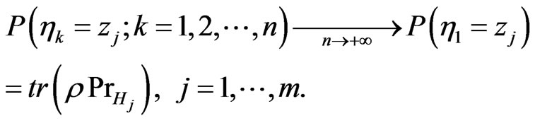
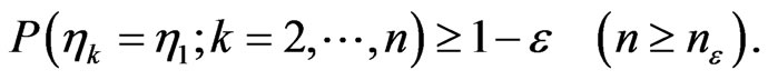
Corollary It holds

That does not mean that the state will not be changed in time. This is related to the fact that using only one kind of measurement one cannot determine the state. One can consider a simple example illustrating that. Nevertheless in some special cases one has a total suppression of the time evolution in this sense that the state is not changing.

1.5. Example—A. Turing

Remember the statement of A. Turing: If a system starts in an eigenstate of some observable, and measurements are made of that observable times a second, then the probability that the system will be in the same state after, say, one second, tends to one as tends to infinity.

That we obtain specializing as follows: Let be a state related to a normalized, and let the measurements be related to the selfadjoint operator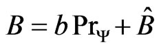, where is a selfadjoint operator such that and are orthogonal, and the eigenvalues of are different from. Then represents an eigenstate of the operator B related to the eigenvalue.

Now, one has to perform measurements according to at the times

Then we have,. Again denotes the random output of the measurement at time.

Then using the corollary mentioned above we obtain

Because is an eigenstate of related to the eigenvalue we have

Thus we can conclude

That implies

Because of the random value would represent the output of a measurement at time and the event “ “ means that at time the system would be in the initial state. Thus we can conclude that the probability that at time the system will be in the same state as at the beginning tends to one as tends to infinity.

1.6. Example—Arrow Paradox

In quantum mechanics one uses the Hilbert space in order to describe a quantum particle located in the space. Now, again let be a pure state related to a normalized wave function. We interpret as the state of the arrowhead at time, and we assume that the wave function is concentrated on a “very small region”, thus the position of the arrowhead at time 0 is “almost fixed”.

Now, let be the space of the wave functions concentrated on. We specialize. Then the corresponding measurement means: “checking whether the arrowhead will be inside of the region or not”. Consequently the event “” means that “at time the arrowhead is located inside of the region”.

Because of the corollary mentioned above may be rewritten as follows

i.e., the arrow will not move under “continual observation”.

1.7. Can We Use the Quantum Zeno Effect in Order to “Prove” That the Brain Acts Like a Quantum System?

More and more specialists in life science are convinced that one should use quantum models in order to describe some special bio-systems, others are against quantum models. Now we want to propose a certain experiment that may be helpful to decide whether a concrete system behaves like a quantum system or not.

The basic idea is as follows: First perform a sequence of measurements with very high frequency, i.e., the length of the time series obtained within, say, one second is very large. Then produce a time series where is very small (e.g.). Now, compare the correlations and. In the idealistic quantum case it would be because of the quantum Zeno effect. But that is not realistic because of certain classical noise caused by the measuring procedure. Nevertheless, in the quantum case should be significant lower than—which would contradict to the classical case.

Finally let us mention that some parts of this paper are based on [21].

2. Distribution of a Time Series Related to Quantum Measurements

Let be a semigroup of unitary operators on a separable Hilbert space representing the time evolution of a quantum system. denotes the state of the quantum system at time.

We consider a sequence of times and perform measurements at time related to selfadjoint operators given by their unique representation

i.e., represents an orthogonal decomposition of and if . Formally the random outputs of these measurements we identify with random numbers.

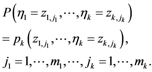
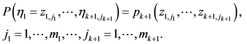
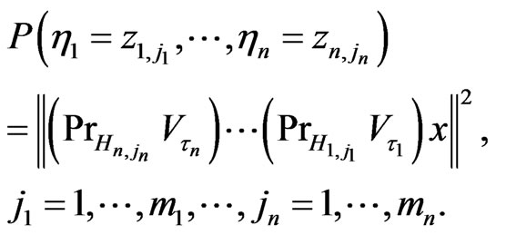
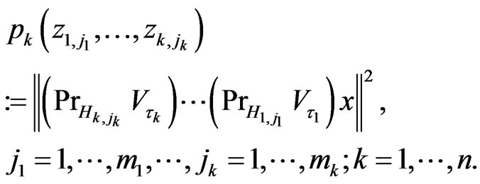
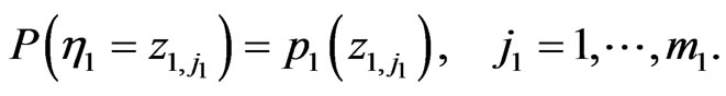
Theorem 1 Let be a pure state related to,. Further we put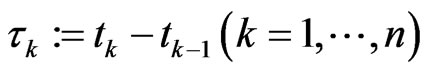. Then we get the probabilities

Proof 1 We put

(2.1)

Then we get

(2.2)

Now let us assume that for some it holds

(2.3)

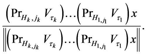
Using J. von Neumann’s rule we can conclude that under condition “” (i.e., knowing the exact results of the measurements) immediately after the -th measurements the quantum system is in the pure state

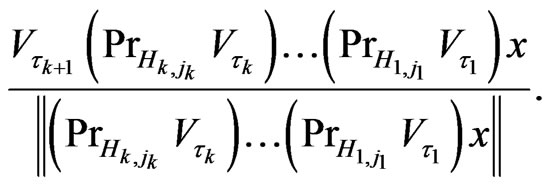
Then at time the system is in the state

Now performing the measurement according to we get the value with (conditional) probability

(2.4)

Using (2.1), (2.3) and (2.4) we obtain

That proves Theorem 1.

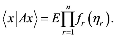
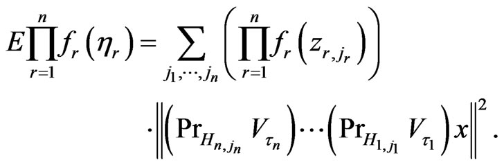
Now let be measurable functions. We will consider the expectation

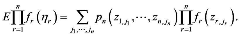(2.5)

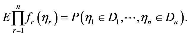
Example 1 Let be measurable subsets of R. We consider the indicator functions. Then we have

Example 2 We consider the case,. Then we have

Example 3 We consider the case . Then we have

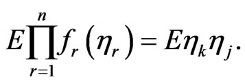
Using Example 2 and Example 3 we can calculate correlations.

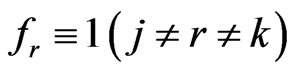
Example 4 We consider the case

.

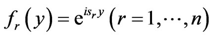Then

represents the characteristic function of the vector. Observe that these characteristic functions represent the complete information concerning the distribution of time series.

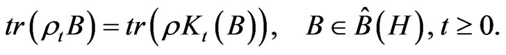
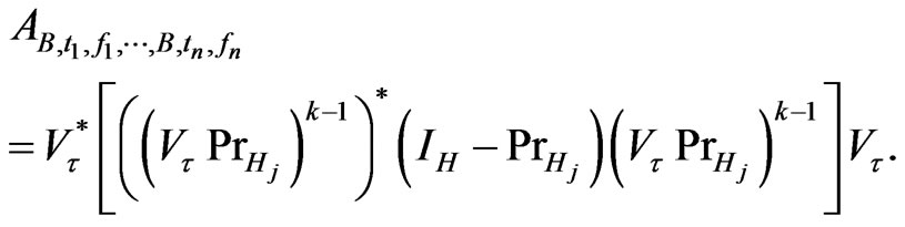
Now in quantum mechanics expectations are of the type where represents the state of the system and is a certain (selfadjoint) operator. For that reason we will construct an operator related to such that we obtain

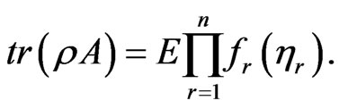(2.6)

For that purpose we define the following linear mappings from the set of bounded operators on into this set putting

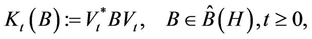(2.7)

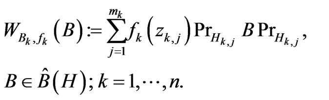(2.8)

Then we put

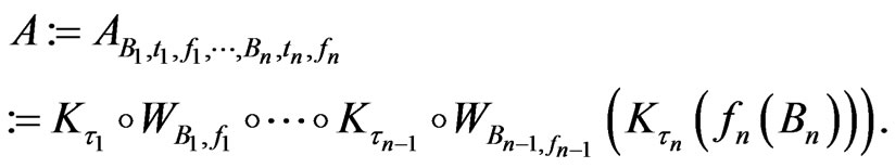(2.9)

If the operator is selfadjoint then is selfadjoint. Further one easily checks that is selfadjoint if is selfadjoint and is a real function. For that reason we can conclude that the operator is selfadjoint if are real functions.

Immediately from the definition of we get

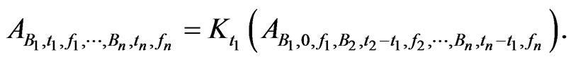(2.10)

Finally we obtain the following theorem.

Theorem 2 Let the operator be given by (2.9). Then (2.6) holds.

Proof 2 We can restrict ourselves to the case of a pure state related to,. Then we have to prove that it holds

(2.11)

Using Theorem 1 and (2.5) we get

(2.12)

Further we have

(2.13)

Finally using (2.13), (2.12), (2.9), (2.8) and (2.7) we obtain (2.11). That proves theorem 2.

Remark 1 The time evolution of a quantum mechanical system usually is characterized by a semigroup of unitary operators. Then the state of the system at time is characterized by

(2.14)

If in addition to that time evolution there are measurements like in the case we have considered this “perturbed” evolution in general no longer may be described by a semigroup of unitary operators. Though the ansatz (2.14) still makes sense. One has to replace the semigroup by a family of completely positive linear maps on. In the case considered above these maps are defined as follows:

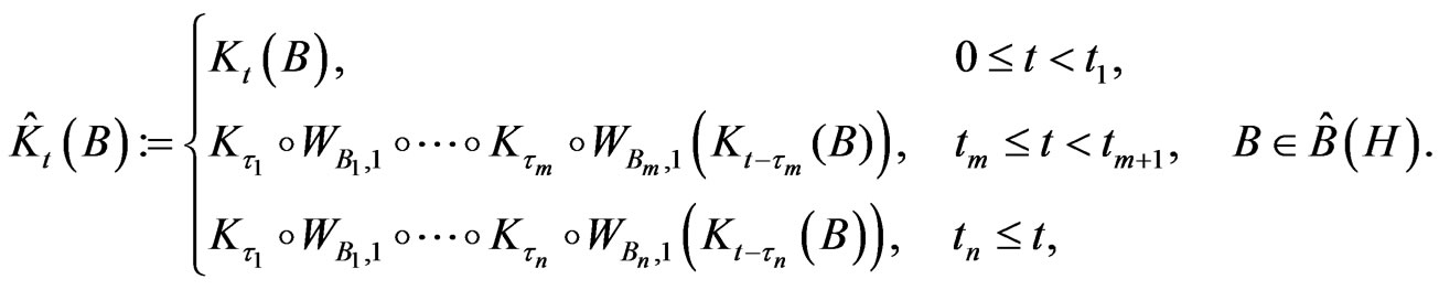(2.15)

Further let us mention that one can generalize our considerations replacing from the beginning the semigroup by an arbitrary semigroup of identity preserving completely positive linear maps on.

Remark 2 Let us consider the trivial case of a time evolution

(2.16)

Further we consider the case of only two measurements, i.e.,. Then we obtain the probabilities

(2.17)

The procedure may be interpreted as follows: first perform a measurement according to and then perform a measurement according to.

Now we change that order, i.e., first perform a measurement according to and then perform a measurement according to. Then we obtain the probabilities

(2.18)

If and commute then we get like in the classical case

(2.19)

In that case specialists say (cf. [22,23]) that “there exist joint probabilities”. If and do not commute one cannot expect that (2.19) holds in general, i.e., for all states. That situation is related to what specialists call “breaking the classical probability law”.

In the following some comments: From (2.17) and (2.18) we obtain two probability measures and on related to two random vectors each of them consisting of two components. In both cases we can define the following (classical) conditional probabilities

(a) “distribution of second component under condition we know the first component”

(b) “distribution of first component under condition we know the second component”

The conditional distributions (a) makes sense from the practical point of view. It represents the behaviour of the output of the second measurement under condition that we know the output of the first measurement. The conditional distribution of the first measurement under condition that we know the output of the second measurement (case (b)) may be senseless because the first measurement has already been done.

Furthermore, one has to take into account that and describe two different procedures. For that reason it seems to be obvious that using conditional probabilities calculated according to for calculations based on will cause some trouble, i.e., basic formulas from classical probability will be violated if.

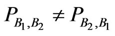Nevertheless, from the mathematical point of view it is interesting to check whether one has joint probabilities because in that case one can apply formulas from classical probability like Bayes formula.

3. On the Quantum Zeno Effect

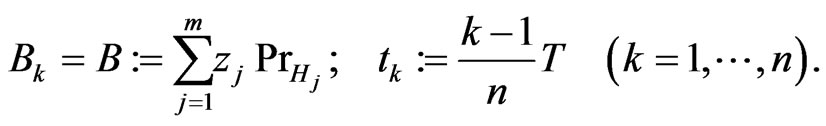
Starting with the notations used in the previous section we will specialize

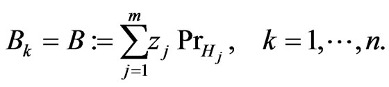(3.1)

(3.2)

That means we consider repeated measurements in the time interval according to starting at time with distance of time

(3.3)

Further we consider the following semigroup of unitary operators on

(3.4)

where the selfadjoint operator is given by its unique representation

(3.5)

i.e., represents an orthogonal decomposition of

and if.

Again denotes the state of the quantum system at time 0, and the random numbers represent the outputs of measurements.

Then we obtain the following theorem.

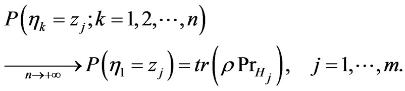
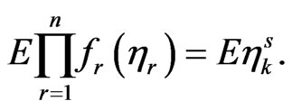
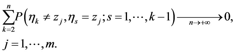
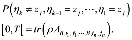
Theorem 3 It holds

(3.6)

Immediately from theorem 3 we get the following corollary.

Corollary 1

(3.7)

Proof of Theorem 3:

We have

(3.8)

For that reason (3.6) is equivalent to

(3.9)

Now we fix, , and define indicator functions putting

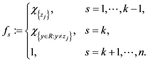(3.10)

Then we get (cf. (2.9))

(3.11)

Further because of Theorem 2 we have

(3.12)

Proving Theorem 3, we can restrict ourselves to the case of a pure state related to,.

Then using (3.11) and (3.12) we obtain

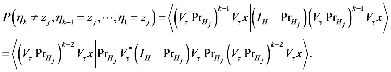(3.13)

Using (3.4) and (3.5) we get

That implies

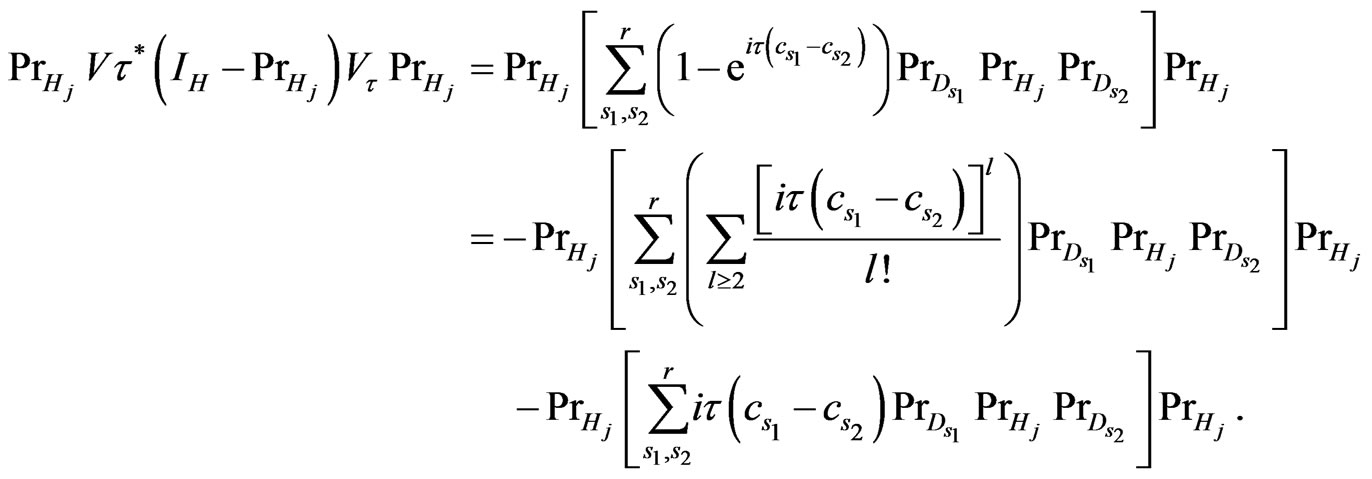(3.14)

Easy calculations show

(3.15)

Because of we obtain using the Schwartz inequality

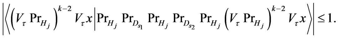(3.16)

Now using (3.3), (3.13), (3.14), (3.15) and (3.16) we can estimate

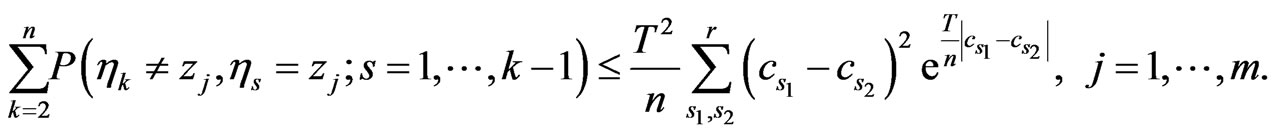(3.17)

That implies (3.9) what proves Theorem 3.

Remark 3 Using (3.8) and (3.17) we obtain

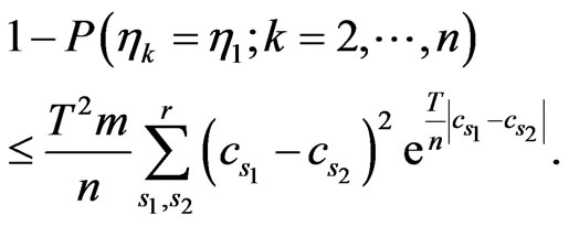
Thus for given we can calculate such that always holds

REFERENCES

- E. C. G. Sudarshan and B. Misra, “The Zeno’s Paradox in Quantum Theory,” Journal of Mathematical Physics, Vol. 18, No. 4, 1977, pp. 756-763.
- T. Nakanishi, K. Yamane and M. Kitano, “AbsorptionFree Optical Control of Spin Systems: The Quantum Zeno Effect in Optical Pumping,” Physical Review A, Vol. 65, No. 1, 2001, Article ID: 013404. http://dx.doi.org/10.1103/PhysRevA.65.013404
- P. Facchi, D. A. Lidar and S. Pascazio, “Unification of Dynamical Decoupling and the Quantum Zeno Effect,” Physical Review A, Vol. 69, No. 3, 2004, Article ID: 032314. http://dx.doi.org/10.1103/PhysRevA.69.032314
- A. Degasperis, L. Fonda and G. C. Ghirardi, “Does the Lifetime of an Unstable System Depend on the Measuring Apparatus?” Il Nuovo Cimento A Series 11, Vol. 21, No. 3, 1974, pp. 471-484. http://dx.doi.org/10.1007/BF02731351
- C. Teuscher and D. Hofstadter, “Alan Turing: Life and Legacy of a Great Thinker,” Springer, Berlin, Heidelberg, 2004. http://dx.doi.org/10.1007/978-3-662-05642-4
- J. von Neumann, “Mathematische Grundlagen der Quantenmechanik,” Springer, Berlin, Heidelberg, 1932.
- K.-H. Fichtner and L. Fichtner, “Bosons and a quantum model of the brain, Jenaer Schriften zur Mathematik und Informatik,” Math/Inf/08/05, Faculty of Mathematics and Informatics, FSU Jena, Jena, 2005, 27 p.
- K.-H. Fichtner and L. Fichtner, “Quantum Models of Brain Activities I—Recognition of Signals,” In: J. C. Garcia, R. Quezada and S. B. Sontz, Eds., Quantum Probability and Related topics, XXIII of QP-PQ: Quantum Probability and White Noise Analysis, World Scientific, New Jersey, London, Singapore, 2008, pp. 135-144.
- K.-H. Fichtner, L. Fichtner, W. Freudenberg and M. Ohya, “On a Mathematical Model of Brain Activities,” Quantum Theory, Reconsideration of Foundations-4, 962 of AIP Conference Proceedings, American Institute of Physics, Melville, New York, 2007, pp. 85-90.
- K.-H. Fichtner, L. Fichtner, W. Freudenberg and M. Ohya, “On a Quantum Model of the Recognition Process,” In: L. Accardi, W. Freudenberg and M. Ohya, Eds., Quantum Bio-Informatics, XXI of QP-PQ: Quantum Probability and White Noise Analysis, World Scientific, New Jersey, London, Singapore, 2008, pp. 64-84.
- K.-H. Fichtner, L. Fichtner, W. Freudenberg and M. Ohya, “On a Quantum Model of the Brain Activities,” In: L. Accardi, W. Freudenberg and M. Ohya, Eds., Quantum Bio-Informatics III, XXVI of QP-PQ: Quantum Probability and White Noise Analysis, World Scientific, New Jersey, London, Singapore, 2010, pp. 81-92.
- K.-H. Fichtner, L. Fichtner, W. Freudenberg and M. Ohya, “Quantum Models of the Recognition Process—On a Convergence Theorem,” Open Systems and Information Dynamics, Vol. 17, No. 2, 2010, pp. 161-187. http://dx.doi.org/10.1142/S1230161210000114
- K.-H. Fichtner, L. Fichtner, W. Freudenberg and M. Ohya, “Self-Collapses of Quantum Systems and Brain Activities,” In: L. Accardi, W. Freudenberg and M. Ohya, Eds., Quantum Bio-Informatics IV, XXVIII of QP-PQ: Quantum Probability and White Noise Analysis, World Scientific, New Jersey, London, Singapore, 2011, pp. 101-115.
- K.-H. Fichtner, L. Fichtner, K. Inoue and M. Ohya, “Internal Noise Caused by the Memory,” Open Systems and Information Dynamics, Vol. 18, No. 4, 2011, pp. 405- 422. http://dx.doi.org/10.1142/S1230161211000285
- K.-H. Fichtner, K. Inoue and M. Ohya, “On a Quantum Model of Brain Activities—Distribution of the Outcomes of EEG-Measurements and Random Point Fields,” Open Systems and Information Dynamics, Vol. 19, No. 4, 2012, Article ID: 1250025.
- J. M. Schwartz, H. P. Stapp and M. Beauregard, “Quantum Physics in Neuroscience and Psychology: A Neurophysical Model of Mind-Brain Interaction,” Philosophical Transactions of the Royal Society of London B, Vol. 360, No. 1458, 2005, pp. 1309-1327. http://dx.doi.org/10.1098/rstb.2004.1598
- R. Penrose, “The Emperor’s New Mind: Concerning Computers, Minds and The Laws of Physics,” Oxford University Press, Oxford, 1989.
- S. Hameroff and R. Penrose, “Orchestrated Objective Reduction of Quantum Coherence N Brain Microtubules: The ‘Orch OR’ Model Forconsciousness,” Mathematics and Computer Simulation, Vol. 40, No. 3-4, 1996, pp. 453-480. http://dx.doi.org/10.1016/0378-4754(96)80476-9
- R. Hari and O. V. Lounasmaa, “Neuromagnetism: Tracking the Dynamics of the Brain,” Physics World, Vol. 13, 2000, pp. 33-38.
- W. Tirsch, “Biomedizinische Relevanz der quantitativen EEG Analyse,” LMU München, München, 2009.
- K.-H. Fichtner, “Time Series Related to Quantum Measurements and the Quantum Zenon Effect,” Jenaer Schriften zur Mathematik und Informatik, Math/Inf/02/ 2012, Faculty of Mathematics and Informatics, FSU Jena, Jena, 2012, 15 p.
- M. Asano, M. Ohya, Y. Tanaka, A. Khrennikov and I. Basieva, “Quantum Like Representation of Baysian Updating,” American Institute of Physics, Vol. 1327, No. 1, 2011, pp. 57-62.
- M. Asano, I. Basieva, A. Khrennikov, M. Ohya and I. Yamato, “A General Quantum Information Model for the Contextual Dependent Systems Breaking the Classical Probability Law,” ArXiv:1105.4769v1(quant-ph), 21 May 2011.