Applied Mathematics
Vol.4 No.5A(2013), Article ID:31907,8 pages DOI:10.4236/am.2013.45A008
Finite Element Analysis in Combination with Perfectly Matched Layer to the Numerical Modeling of Acoustic Devices in Piezoelectric Materials
1TDK, Sophia Antipolis, France
2Institut Femto-st, Besançon, France
3TDK, Munich, Germany
Email: karim.dbich@femto-st.fr
Copyright © 2013 Dbich Karim et al. This is an open access article distributed under the Creative Commons Attribution License, which permits unrestricted use, distribution, and reproduction in any medium, provided the original work is properly cited.
Received March 1, 2013; revised April 23, 2013; accepted April 30, 2013
Keywords: Finite Element Method; Perfectly Matched Layer; Surface Acoustic Wave; Piezoelcetric; Numerical Modeling
ABSTRACT
The characterization of finite length Surface Acoustic Wave (SAW) and Bulk acoustic Wave (BAW) resonators is addressed here. The Finite Element Analysis (FEA) induces artificial wave reflections at the edges of the mesh. In fact, these ones do not contribute in practice to the corresponding experimental response. The Perfectly Matched Layer (PML) method, allows to suppress the boundary reflections. In this work, we first demonstrate the basis of PML adapted to FEA formalism. Next, the results of such a method are depicted allowing a discussion on the behavior of finite acoustic resonators.
1. Introduction
The ultimate optimization in the development of components such as SAW (Surface Acoustic Wave) and BAW (Bulk Acoustic Wave), is to increase the capability to simulate the real shape of the resonator. In the case of SAW devices, the main effort is currently devoted to account for lateral resonance [1] that can pollute the SAW main contribution exploited for the filtering operation. These phenomena can be adequately modeled using advanced numerical tools, and more particularly a formulation must be developed to allow the analysis of the active part of the resonator as well as the area near the edges, suppress modes generated by the lack of consistent data absorbing conditions.
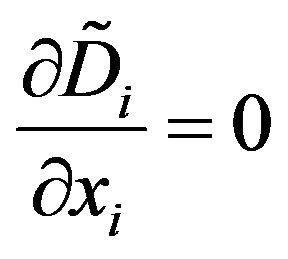
When one solves an equation numerically by volume discretization like in Finite Element Analysis (FEA), one must truncate the computational grid in some way. In such cases, the important thing is how to perform this truncation without introducing significant artifacts into the computation. Two cases may arise. If the computational domain is large enough and the sides are seen by a very attenuated wave so there is no problem. In the other hand, if the wave doesn’t vanish at the mesh boundary we must apply absorbing condition to avoid spurious reflection. The application of boundary conditions as rigid walls (Dirichlet or Neumann) or periodic boundary conditions leads unacceptable artifacts reflections at the edges of the mesh. Therefore, the wave equations require an absorption condition which makes vanish the waves that strike the edges without reflection into the domain of interest. A well known method is the Boundary Element Method [2]. It is based on the calculation of Green’s functions and requires an external approach to the finite element analysis. We propose a method directly included in the FEA formalism: the Perfectly matched Layer (PML).
In 1994, however, the problem of absorbing boundaries for wave equations was transformed in a seminal paper by Berenger [3]. Berenger changed the question: instead of finding an absorbing boundary condition, he found an absorbing boundary layer, as depicted in Figure 1. An absorbing boundary layer is a layer of artificial absorbing material that is placed adjacent to the edges of the grid, completely independent of the boundary condition. When a wave enters the absorbing layer, it is attenuated by the absorption and decays exponentially;
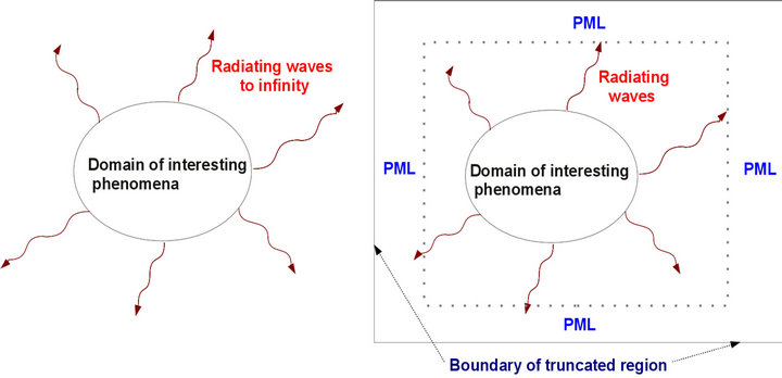
Figure 1. Chematic of the wave problem and the interest of absorbing layer.
even if it reflects o the boundary, the returning wave after one round trip through the absorbing layer is exponentially tiny.
The problem with this approach is that, whenever you have a transition from one material to another, waves generally reflect, and the transition from non-absorbing to absorbing material is no exception so, instead of having reflections from the grid boundary, you now have reflections from the absorber boundary. However, Berenger showed that a special absorbing medium could be constructed so that waves do not reflect at the interface: a perfectly matched layer, or PML. Although PML was originally derived for electromagnetism (Maxwell’s equations), the same ideas are immediately applicable to other wave equations. A lot of work has been devoted to transpose this approach to elasticity problems [4-6].
In the following, we first expose the theoretical development for piezoelectricity-based problems, focusing on the simple case of the scalar plane wave. We will see that the establishment of PML formulation may be described by the combination of the following two steps: first, changing in complex variable, next a coordinate transformation allowing the back to real coordinates.
A first numerical application is achieved in 2D to address the simulation of finite dimension of a SAW resonator with a periodic FEA code. Indeed, up to now, the devices modelings were most often considered as 2D systems infinitely periodic in the direction of propagation and infinite in the perpendicular one. We just demonstrate that it is now possible to take into account the effects due to finite dimension along the direction of propagation.
We also show, the interests of PML method is the case of an 3D SAW devices. This is especially to show the influence of the numerical aperture which was considered as infinite. This also shows the effects of lateral edges of such components.
As a conclusion, we propose different tracks to further optimize the PML approach, particularly for 3D piezoelectric problems.
2. Fundamentals@NolistTemp#2.1. Finite Element Analysis and Piezoelectric Problem
First, we start from the variational formulation of the linear dynamic piezoelasticity problem. Here, the unknowns of the problem are mechanical displacement and electrical potential. This approach has been implemented initially by Tiersten [7] Eernisse [8] and Allik and Hughes [9], pioneers in the use of the finite element method for problems of piezoelectricity. Since then, many authors have explored ways and contributed to their improvement for the analysis of piezoelectric transducers in a general sense [10-14]. The principle of this variational formulation consists in balancing the sum of the kinetic and potential energies into the computation volume with the mechanical and electrical solicitations applied at the chosen edges. We thus obtain the following integral form:
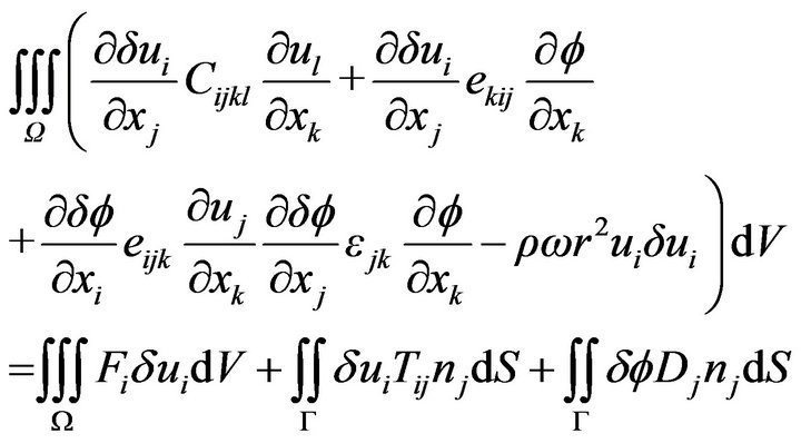 (1)
(1)
The terms 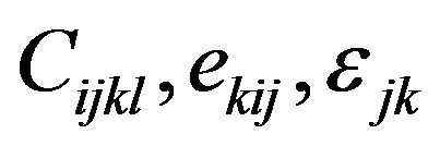 are successively elastic, piezoelectric and dielectric constants.
The method of PML takes care of not changing this formulation. Indeed, we will see that the calculation process leads to change only material constants.
2.2. Perfectly Matched Layers
Let us start with the plane wave  of some wave equation in infinite space.
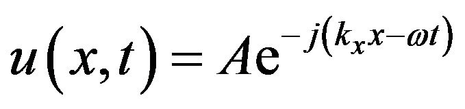 (2)
(2)
In Figure 2, the regions of interest are around the origin  and extended until
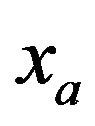 . In particular, we will focus on the problem in the
  direction (the other directions will follow by the same technique). An absorbing domain (PML domain, the blue one in Figure 2) is added on the side edges of the main mesh from
  to
to .
.
The PML setting occurs in four conceptual steps, summarized as follows:
• Changing x in complex variable;
• Coordinate transformation allowing back to real x;
• Transformation of equations in real coordinates into complex materials constants;
• Optimization of PML parameter and construction of the PML region.
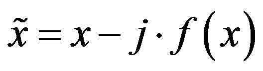
2.3. Changing X in Complex Variable
The first step is to proceed to change of variable complex within the whole domain, which transforms the oscillating waves in exponentially decreasing wave in the PML area without reflections at the interface with the main domain (depicted by the dashed line at  in Figure 2). Since it must not modify the propagation phase, this transform can be written:
 (3)
(3)
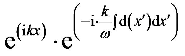
where  growths from the origin of the absorbing area to its end along a defined rate. In the main domain, this function is zero thus there is no changes on the FEA solution). It is clear that the change of variable has the effect of introducing an evanescence of the wave in the PML part. The wave model becomes:
 (4)
(4)
However, since this transform must be efficient for any frequency (we represent the problem in the spectral domain), it is sense to define this function as follows:
 (5)
(5)
We will see thereafter the absorption function  that has been chosen and the criteria imposed.
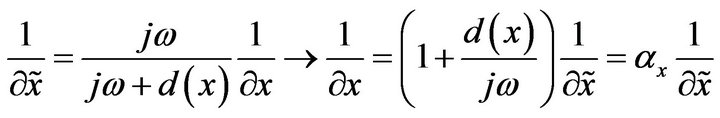
2.4. Coordinate Transformation Which Allow Back to X Real
The second step, is to perform a coordinate transformation to express the complex x as a function of a real coordinate. We can easily define the Jacobian transformation linking the considered coordinate systems as following:
 (6)
(6)
The entire process of PML can be conceptually summed up by this previous transformation of the dierential equation: In the PML aeras where , the oscillating solutions turn into exponentially decaying ones.
In the region of interest 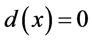 and
and , so the solution remains unchanged even though the change of variable is applied. This is one reason why we do not create reflections at the interface
 .
.
The choice to write the absorbing function with a frequency depedance is motived by looking at what happens for the plane wave :
:
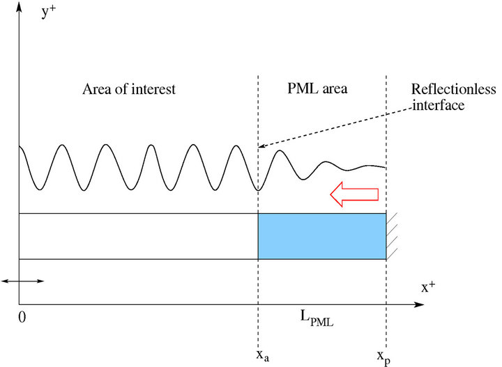
Figure 2. Scheme of PML principle and space domain parting in the x > 0 direction. xa and xp are respectively the lower and upper limits of the PML.
 (7)
(7)
The term  is equal to
 , the inverse of the phase velocity
  in the x direction. This allows that the attenuation rate of the PML is independent of the frequency ω: all wavelengths decrease at the same rate.
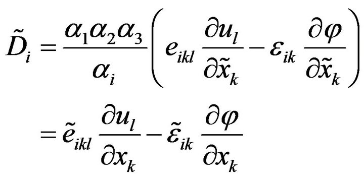
2.5. Tranformation of Equations in Real Coordinates into Complex Materials Constants
Conformably to Zheng and Huang [5], we develop a formulation based on the usual piezoelectricity equations, yielding significant modifications of the elastic, piezoelectric and dielectric constants to account for the absorption.
We now rewrite the elasticity equations in the absorbing region turning x to , using then (6) to express the result in the initial coordinates. In the new coordinates, we have real coordinates and complex materials constants.
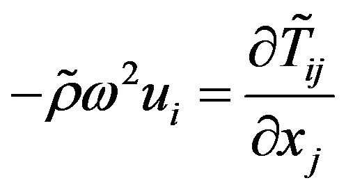
As in [5], the absorbing effect is assumed along the three space directions for the sake of generality. The equilibrium equation then reads:
 (8)
(8)
where  is characterised by its specific function
 .
.  and ui respectively represent the dynamic stresses and displacements, and ρ is the mass density.
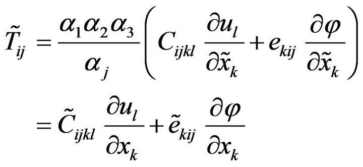
We introduce a non symmetrical stress tensor, expressed in the transformed axis:
 (9)
(9)
where  is the transformed elastic constant tensor relative to the absorption area. We multiply (8) by
 , thus yielding Newton relation for PMLs in the real coordinates
 (10)
(10)
where 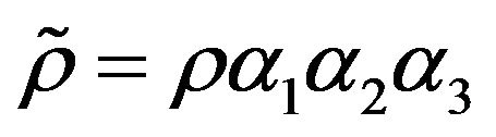 is the mass density relative to the transformed domain. Given that the obtained form of the equilibrium equation complies with the classical expression for usual solids, it is allowed to exploit the standard FEA formulation. It must however be careful to take into account the frequency dependence of the transformed tensors (stress and electrical displacement) in the PML région. These developments of course can be extended to piezoelectricity by rewriting Poisson’s equation and taking into account the piezoelectric coupling in the stress definition as follows:
 (11)
(11)
Poisson’s equation expressed in the transformed system of axes reads:
 (12)
(12)
with 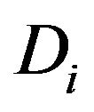 the electrical displacement vector. To provide an homogeneous formulation, we proceed as for the stress definition (9), multiplying the electrical displacement by
 , yielding:
 (13)
(13)
As for the propagation Equation (8), the Poisson’s condition is written accounting for these changes as:
 (14)
(14)
In the same way as the transformation of the stress tensor, we introduce the modified piezoelectric and dielectric constants defined as follows:
 (15)
(15)
We now are able to establish a FEA formulation exploiting these developments in Equation (16) without fundamental changes of the variational formulation developed in Equation (1):
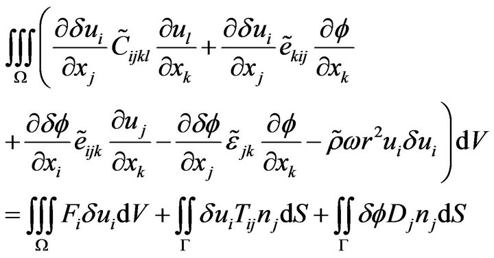 (16)
(16)As some care must be paid to the truncation of the computational region and also to the choice of the absorption function, next paragraphs are dedicated to these questions.
2.6. Optimization of PML Parameter and Construction of the PML Region
Once we have performed the PML transformation of the FEA formulation, the solutions are unchanged in the region of interest  and exponentially decaying in the PML regions
 . At the end of the PML domain, the boundary conditions are not important. Indeed, even if a hard wall is set on this frontier, the reflected waves on it can be neglected after the propagation into the PML.
In order to optimize the operation of the PML, the absorption function  must be wisely chosen. We discuss here the absorption function and the importance of its parameters.
In our developments, the absorption function is chosen to avoid introducing any brutal change in the physical constants. That must be applied as well at the interface between the main domain and PML domain as throughout the PML area. This signifies it must exhibits derivatives close to zero at each edge of the PML area, but it must continuously vary more rapidly within this area to avoid meshing a too long PML zone. We also want this function to be even (symmetrical) so it can apply on the both sides of a domain centred around . As proposed in [6], we consider the following form of
  that allows to match all these specifications at once
 (17)
(17)
with xa and xp the limits of the PML area and n an integer controlling the absorption rate. The coefficient  is an adjustable normalisation parameter. This function is plotted in Figure 3 to show its compliance to the above definition.
With , the first derivates are not zero. So the matching coditions are not observed. On the other hand, for n too large (for instance, n equal to 4 or 5), the slope in the middle of the PML is high and this can lead to numerical reflections. Indeed, in the FEA formalism, the absorbing function must be numerically integrated on

Figure 3. Comparison between different absorption rates of the function d(x). The parameter dmax is equal to 4.
each elements of the mesh. So, considering Gauss rules, a high order polynomial requires more points to converge. If this condition is not respected, some artifacts may appear.
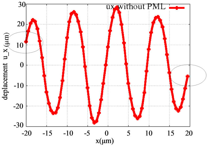
To highlight, the effects of the pml, Figures 4(a) and (b) depict the case without and with PML. We see in Figure 4(b) that the mechanical displacement becomes close to zero at the end of the PML area by decreasing continualy. Unlike in case without PML where the mechanical displacement does not decay.
In Figure 5, the influence of dmax on the displacement is demonstrated in the PML domain. We can see the importance of choosing the parameter  to obtain coherent behavior of PML. For
 , the absorbing function reveals a smoothy behavior providing a constant decreasing of the wave .along the PML. In contrast, for
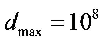 , we see that the displacement seems to be inconsistent. This is due to the fact that the increase of
  leads to a too brutal change in the rate of absorption and induces numerical reflections.
 (a)
(a)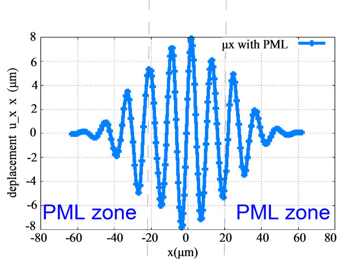 (b)
(b)
Figure 4. (a) x displacement along the whole domain without PML. (b) Attenuation of the mechanical displacement along the PML zone and main domain.

Figure 5. Behavior of the displacement along the PML region for two different parameters dmax: dmax=106 (in dark blue) and dmax=108 (in light blue).
The PML/FEA formalism is achieved for each frequency point and so is time consuming. Then for practical application, we chose  as the best trade-off between a strong absorption rate and fast computations. The dmax is selected between 106 and 107.
3. Numerical Tests and Validation
The efficiency of the PML implemented in FEA is depicted in three parts. First, a 2D-case is investigated showing the absorbing due to the PML domain and the effects of the effects of the finite lateral size on the behavior of a SAW resonator. Next, the same study is repeated but in a 3D configuration in order to validate the general PML approach. At last, a realistic SAW problem is addressed by considering the aperture of the resonator and absorbing the lateral leaky modes. First, A 2D SAW resonator problem is addressed. The geometrical configuration is depicted in Figure 6. A piezoelectric medium (quartz YXl/36) is driven by 4 pairs of electrodes. The electrodes are non massive and alternatively activated with  and
and . The period is 10 µm. The depth of PML on both sides is 35 µm. The hight of the mesh is 75 µm. The absorbing parameters are set to
  and
and .
.
The result of this simulation is shown in Figure 7. We depicted the vibrations for the x-displacements in the XY plane. The vibrations in both the right and left PML domains are strongly reduced as and as they enter into. The decreasing factor is around 10−5. We also hardly observed the phenomena of diffraction due to the finite lateral size of the resonator. Indeed, weak lobes appears at the both lateral end of the grating and give rise to bulk wave and so losses in the medium. Next, we repeat the same simulation as the one depicted in Figure 6 but for a 3D geometry. The configuration is drawn in Figure 8. The piezoelectric is once more quartz YXl/36. The same set of non massive electrodes is still powered in the same
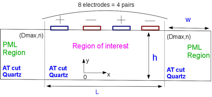
Figure 6. Characteristic configuration for finite SAW resonators considering the mixed PML/FEA approach. Eight non massive electrodes are activated alternatively (V1 = 1V, V2 = 0V). The width of electrodes is equal to 2.5µm and the period of the resonator is set to 10 µm. The piezoelectric medium is quartz YXl/36. Its thickness vary from zero. On the left and right parts of the scheme, two PML domains are set. No boundary conditions are defined neither at the top nor at the bottom. Th depth of the piezoelectric h is chosen to avoid any interaction with the penetrating bulk wave at the bottom interface. dmax = 106 and n = 3.
x-Displacemen (m) with PML

Figure 7. The vibrations for x-displacement in the XY plane for the 2-D problem depicted in Figure 6. The piezoelectric medium is quartz YXl/36 activated by eight electrodes alternatively powered by V = 1 V and V = 0 V The PML domains are delimited by the white dashed line at the let and right sides. The frequency is 318 MHz. h = 7e−5 m, dmax = 106 and n = 3.

Figure 8. Same configuration as in Figure 6 but in 3D-case. The z-direction is periodically infinite. So the electrodes are infinitly long in the z-direction.Eight non massive electrodes are activated alternatively (V1 = 1V, V2 = 0V). h = 7e−5 m, dmax = 106 and n = 3.
way. The absorbing conditions are also the same. The x-displacement obtained by FEA/PML is shown in the perspective Figure 9.
It is clearly demonstrated that the vibration have the same absorption as in the 2D-case even if the absorbing factor is slightly worse. One more time, the losses in the medium can also be observed at the end of the resonator. We notice that there is no reflection at the end of the mesh for both side edges and bottom boundaries. The last configuration highlight a new point to design SAW resonator. Indeed, up to now, the devices modelings were most often considered as 2D systems infinitely periodic in the direction of propagation and infinite in the perpendicular one. We just demonstrate that it is now possible to take into account the effects due to finite dimension along the direction of propagation. In this part, we depict the way to address the problem of real aperture of a SAW resonator. In other words, we consider a finite dimension in the perpendicular direction of the propagation. In this study, the number of electrodes is infinite. The geometrical configuration is depicted in Figure 10. The materials properties, excitation and dimensions of the grating are still the same as previously in Figure 8.
We now consider a length of the electrodes equal to 54 µm for a period in the direction of propagation equal to 10 µm. The buses on the both right and left gratings are infinite along the propagation and 20 µm wide. We also assume that the piezoelectric medium continue towards the infinity on the both sides of the resonator. The PML method allows this assumption. Once again, we show the vibration for the x-displacement in the perspective Figure 11. The factor of absorption is still very high even if we notice a slight decrease. The Ω domain stands for the

Figure 9. The vibrations for x-displacement for the 3-D problem depicted in Figure 8. The piezoelectric medium is quartz YXl/36 activated by eight electrodes alternatively excited by V = 1 V and V = 0 V. The PML domains are delimited by the white dashed line at the let and right sides. The frequency is 318MHz. h = 7 e−5 m, dmax = 106 and n = 3.
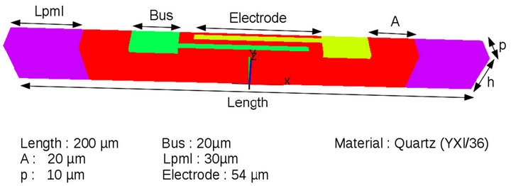
Figure 10. Configuration of an infinitely periodic SAW resonator in the propagation direction but with finite lateral dimension. The z-direction is infinitely periodic and the non massive electrodes are alternatively excited with V1 = 1 V and V2 = 0 V. The piezoelectric medium is quartz YXl/36. The length of electrodes is 54 µm while the period is 10 µm. h = 30 µm, dmax = 106 and n = 3.
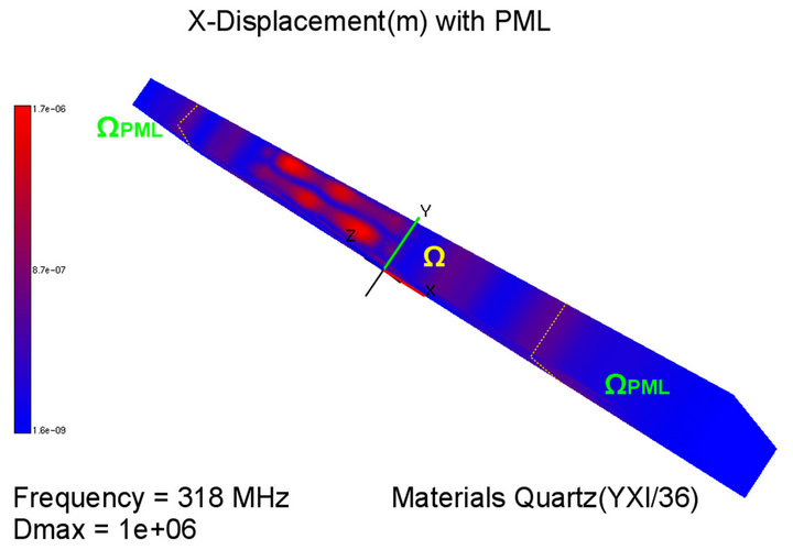
Figure 11. The vibrations for x-displacement for the 3-D problem depicted in Figure 10. The piezoelectric medium is quartz YXl/36 activated by electrodes excited by V = 1 V and V = 0 V. The PML domains are delimited by the white dashed line at the let and right sides. The frequency is 318 MHz. h = 30 µm, dmax = 106 and n = 3.
physical space in which the SAW is generated. We observe the Rayleigh wave in the middle of Ω. On each side of this vibration, the presence of the buses is denoted by two maxima of displacement. These displacements give rise to a lateral mode which is reflected on the side edges if there is no activated PML. But, in Figure 11, all PML are turned on. So, the lateral modes can be detected at the very end of the Ω area, just before the PML domains. However, due to the presence of the PML, this mode does not reflect on the side edges and moreover its amplitude decreases at the time it progress in the PML from the beginning to the end where it almost vanishes by them.
These three results show the efficiency of the combining of PML and FEA to simulate the effects due to the consideration of the real length or width of a SAW resonator. Thus, using this kind of method, we are able to simulate realistic effects in SAW. This method can also be applied to other kind of resonator.
4. Conclusion
Perfectly Matched Layer method has been developed for wave equations: elastics wave in solids and piezoelectric materials. This is, in the context of a periodic Finite Element Analysis code. In this work, we demonstrated a PML method well adapted to the FEA. The ability to absorb the outgoing wave from a resonator has been highlighted for different configurations. First, a 2D-system of SAW resonator was address and we noticed that all the waves going into the PML are absorbed. The lobes of diffraction due to the ends of the grating were also observed. Next, the comparison between the 2D-results and 3D-ones in the same configuration allow us to validate complete PML approach. At last, we displayed the influence of the lateral modes for a real model of SAW resonator considering the length of the electrodes as well as the buses. We must also note that this absorbing method could be coupled with the BEM to consider most configurations for any kinds of acoustics devices.
REFERENCES
- M. Solal, S. Ballandras and V. Laud, “A P-Matrix Based Model for SAW Grating Waveguides Taking into Account Modes Conversion at the Reflection,” IEEE Transactions on UFFC, Vol. 51, No. 12, 2004, pp. 1690-1696.
- T. Laroche, M. Mayer, X. Perois, W. Daniau, J. Garcia, S. Ballandras and K. Wagner, “Mixed Finite Element Analysis/Boundary Element Method Based on Canonical Green’s Function to Address Non-Periodic Acoustic Devices,” 2011 Proceeding of Ultrasonics Symposium (IUS), Orlando, 2011, pp. 1850-1853.
- J. P. Bérenger, “A Perfectly Matched Layer for the Absorption of Electromagnetic Wave,” Journal of Computational Physics, Vol. 114, No. 2, 1994, pp. 185-200. doi:10.1006/jcph.1994.1159
- D. Komatitsch and J. Tromp, “A Perfectly Matched Layer Absorbing Boundary Condition for the Second-Order Seismic Wave Equation,” Geophysical Journal International, Vol. 154, No. 1, 2003, pp. 146-153. doi:10.1046/j.1365-246X.2003.01950.x
- Y. B. Zheng and X. J. Huang, “Anisotropic Perfectly Matched Layers for Elastic Waves in Cartesian and Curvilinear Coordinates,” MIT Earth Resources Laboratory Industry Consortium Report, Massachusetts Institute of Technology, Earth Resources Laboratory, 2002.
- D. Appelö, “Absorbing Layers and Non-Reflecting Boundary Conditions for Wave Propagation Problems,” Ph.D. Thesis, KTH Royal Institute of Technology, Stockholm, 2005.
- H. F. Tiersten, “Hamilton’s Principle for Linear Piezoelectric Media,” Proceedings of the IEEE, Vol. 55, No. 8, 1967, pp. 1523-1524.
- E. P. Eernisse, “Variationnal Method for Electroelastic Vibration Analysis,” IEEE Transactions on Sonics and Ultrasonics, Vol. 14, No. 4, 1967, pp. 153-160. doi:10.1109/T-SU.1967.29431
- H. Allik and T. J. R. Hugues, “Finite Element Method for Piezoelectric Vibration,” International Journal for Numerical Methods in Engineering, Vol. 2, No. 2, 1970, pp. 151-157. doi:10.1002/nme.1620020202
- H. Allik, K. M. Webman and J. T. Hunt, “Vibrational Response of Sonar Transducers Using Piezoelectric Finite Elements,” Journal of the Acoustical Society of America, Vol. 56, No. 6, 1974, pp. 1782-1791. doi:10.1121/1.1903513
- D. Boucher, Y. Lagier and C. Maerfeld, “Computation of the Vibrationnal Modes for Piezoelectric Transducers Using a Mixed Finite Element Pertubational Method,” IEEE Transactions on Sonics and Ultrasonics, Vol. 28, No. 5, 1981, pp. 318-330. doi:10.1109/T-SU.1981.31270
- M. Naillon, R. H. Coursant and F. Besnier, “Analyse de Structures Piézoélectriques par une Méthode des Éléments Finis,” Acta Electronica, Vol. 25, No. 4, 1983, pp. 341- 362.
- W. Steichen, G. Vanderbork and Y. Lagier, “Determination of the Power Limits of a High Frequency Transducer Using the Finite Element Method,” Power Sonic and Ultrasonic Transducers Design, 1988, pp.160-174.
- R. Lerch, “Simulation of Piezoelectric Devices by Two and Three Dimensionnal Finite Elements,” IEEE Transactions on Ultrasonics, Ferroelectrics and Frequency Control, Vol. 37, No. 3, 1990, pp. 233-247. doi:10.1109/58.55314