Applied Mathematics
Vol.4 No.2(2013), Article ID:28200,12 pages DOI:10.4236/am.2013.42048
Analytical Expressions of Concentration of VOC and Oxygen in Steady-State in Biofilteration Model
Department of Mathematics, The Madura College, Madurai, India
Email: *raj_sms@rediffmail.com
Received October 8, 2012; revised November 8, 2012; accepted November 15, 2012
Keywords: Biofilters; Volatile Organic Compounds; Oxygen; Adomian Decomposition Method; Mathematical Modeling; Non-Linear Reaction/Diffusion Equations
ABSTRACT
Mathematical models of steady-state biofilteration are discussed. The theoretical results are much useful for the design of biofilters. This model is based on the system of non-linear reaction/diffusion equations contains a non-linear term related to Monod kinetics, Andrews kinetics, interactive model from Monod kinetics and Andrews kinetics. Analytical expression of concentration of VOC (Volatile organic compounds) and oxygen are derived by solving the system of non-linear equations using Adomian decomposition method (ADM) method. Our analytical results are also compared with the simulation results. Satisfactory agreement is noted.
1. Introduction
Biological system for elimination of volatile organics have been explored on experimental studies [1-3]. However, researches into the theoretical studies regarding biofilter models is rather limited. The pioneering contribution of Ottengraf and co-workers [1,2] of this model is based on some rather simplistic assumptions. The closed analytical expression have been used in validating-scale experimental data and actual design of pilot-scale biofilter units. Recently Zarook et al. [3], extended the work of Ottengraf et al. [1] and presented a detailed steady-state biofilteration model for single volume. Allen and Phatak [4] have extended their model to describe the biofilteration of VOC mixtures under steady-state conditions. Dehusses and Dunn [5] reports a transient biofilteration model which is based on the assumption that oxygen is in excess and the kinetics are of the Michaelis-Menten or Monod type. The steady-state model of Zarook et al. [3] was extended to describe the transient performance [6] of the biofilters. All the steady-state and transient biofilteration models [1-6] are based on the assumption that substrates are transported into the biofilm through diffusion. Biological systems for elimination of VOCs have been explored both on the experimental and mathematical modeling levels primarily in the Netherlands by Ottengraf et al. [6-8] followed by many researches even though land area requirements and lack of process control still restrict the industrial use of these systems. Several researchers [1,3,6,9-13] developed models to predict biodegradability of organic compounds in biofilters. The three general plans for biological treatment systems are biofilters, biotrickling filters and bioscrubbers. In biofilters, the porous medium is kept damp by maintaining the humidity of the incoming air and by occasional sprinkling. The reliability of biological processes and in particular of biofilteration for the treatment of waste gas streams containing VOC has been demonstrated by a very large number of experimental studies.
Recently Zarook et al. [14] obtained the concentration of VOC and oxygen only for the limiting cases (zeroorder kinetics and first-order kinetics) for monoid kinetics. However, to the best our knowledge, no analytical expressions pertaining to the steady state concentrations of VOC, oxygen and effectiveness factor have been reported. The purpose of this paper is to derive the analytical expression of concentration of VOC and oxygen for all values of parameters and all reaction mechanisms, using the Adomian decomposition method.
2. Mathematical Formulation of the Problem
A steady-state biofilteration model (Figure 1) constitutes a set of mass balances within the biofilm. The mass balance equations in the biofilm are [14]:
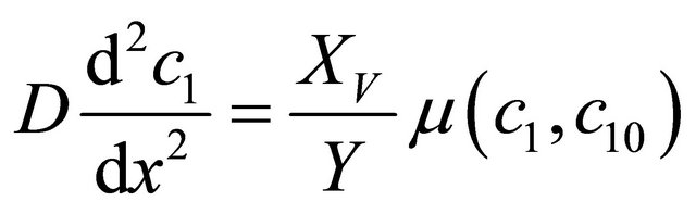 (1)
(1)
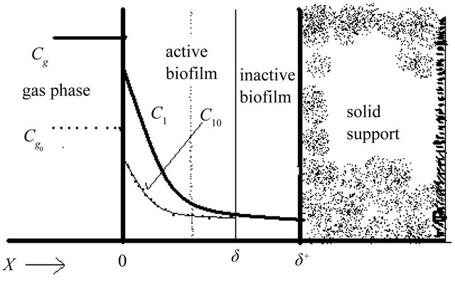
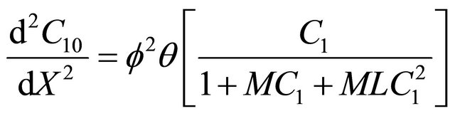
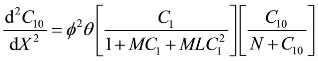
Figure 1. Biofilm concept of the biofilter.
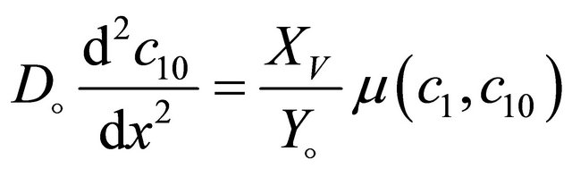 (2)
(2)
with the boundary conditions
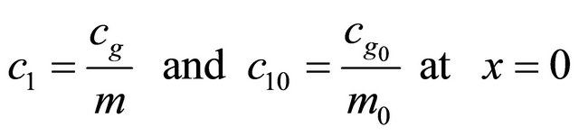 (3)
(3)
 (4)
(4)
where ![]() and
and  are the concentration of VOC and oxygen at a position x in the biofilm,
  and
and  are the effective diffusion coefficient of VOC and oxygen in the biofilm.
  denotes biofilm density,
 ![]() and
and  is the amount of biomass produced per amount of VOC consumed and amount of biomass produced per amount of oxygen consumed. For biological systems, The growth rate
 , for various reaction kinetics are given as follows:
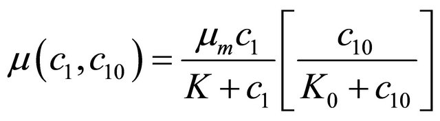
Monod kinetics:
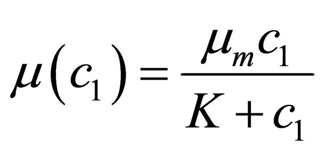 (5)
(5)
Andrews kinetics:
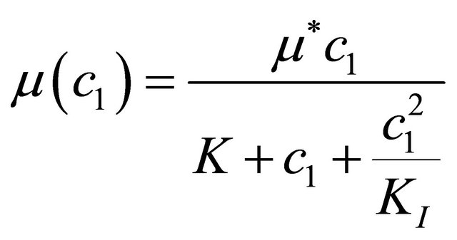 (6)
(6)
When oxygen limits the biodegradation rate, the growth rate is given by interactive model. The above Equations (5) and (6) are written as follows:
Interactive model from Monod kinetics:
 (7)
(7)
Interactive model from Andrews kinetics:
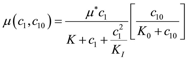 (8)
(8)
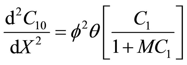
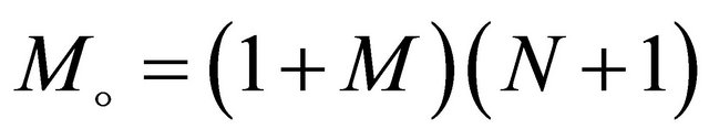
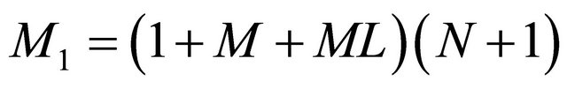
In order to obtain numerical solution of model these equations are brought in dimensionless form through the dimensionless variables and groups. We make the above non-linear partial differential Equations (1) and (2) in dimensionless form by defining the following dimensionless parameters:
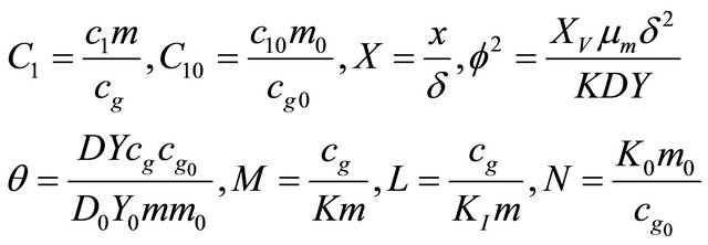 (9)
(9)
where  and
and  denotes the dimensionless concentration of VOC and oxygen, X is the dimensionless position in the biolayer.
  represents the Thiele modulus,
  , M, L and N are dimensionless constants. By substituting the Equation (9) in Equations (1) and (2), we can obtain the following dimensionless non-linear equation for Monod kinetics:
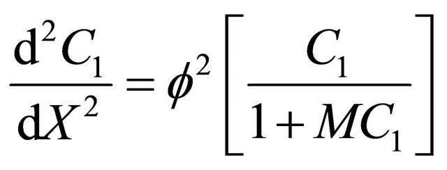 (10)
(10)
 (11)
(11)
Using Equation (9), in the non-linear Equations (1) and (2), we can obtain the following dimensionless nonlinear equation for Andrews kinetics:
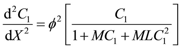 (12)
(12)
 (13)
(13)
Using Equation (9), the dimensionless non-linear equation for Interactive model of Monod kinetics becomes
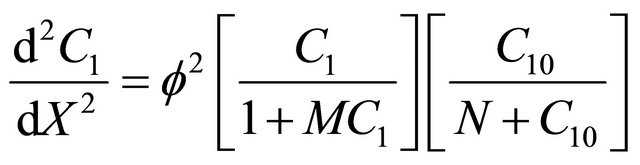 (14)
(14)
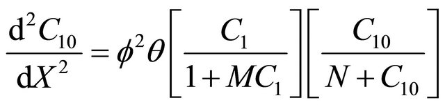 (15)
(15)
The dimensionless non-linear equation for Interactive model of Andrews kinetics of the Equations (1) and (2) is
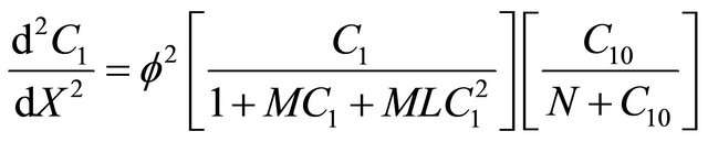 (16)
(16)
 (17)
(17)
Now the boundary condition in dimensionless form may be represented as follows:
 (18)
(18)
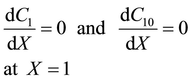 (19)
(19)
For all the above cases, we can obtain the relation between  and
and  as follows:
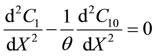
Integrating the above equation twice and using the boundary condition (18) and (19) we get
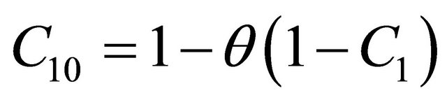 (20)
(20)
When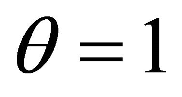 , the concentration of VOC
  and oxygen
  becomes equal. When
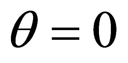 , the concentration of oxygen
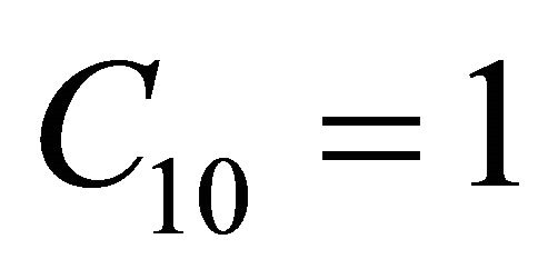 . When
 , the concentration of VOC
  becomes one.
3. Analytical Solutions of the Concentrations Using the Adomian Decomposition Method (ADM)
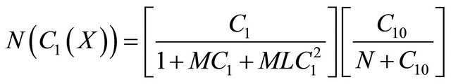
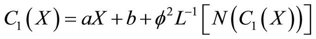
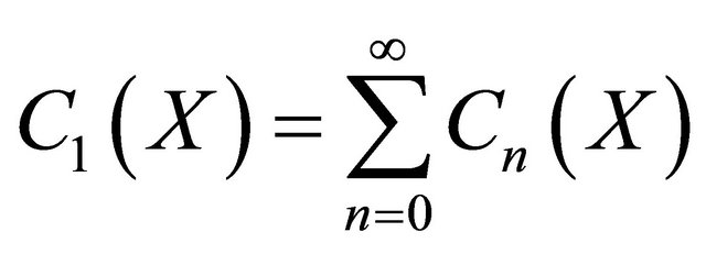
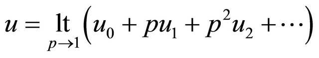
Nonlinear phenomena play a crucial role in physical chemistry and biology (heat and mass transfer, filtration of liquids, diffusion in chemical reactions, etc.). Constructing a particular, exact solution for these equations remains an important problem. Finding an exact solution that has a physicochemical or biological interpretation is of fundamental importance. This model is based on a non-stationary system of diffusion equations containing a nonlinear reaction term. It is not possible to solve these equations using standard analytical techniques. The investigation of an exact solution of nonlinear equations is interesting and important. In the past several decades, many authors mainly paid attention to studying the solution of nonlinear equations by using various methods, such as the Backlund and the Darboux transformation [15,16], the inverse scattering method [17], the bilinear method [18], the tanh method [19], the variational iteration method [20], the HPM [21-25], ADM [26-30]. The ADM was successfully applied to autonomous ordinary differential equations for nonlinear polycrystalline solids and to other fields. This method has been proved by many authors to be a powerful mathematical tool for various kinds of nonlinear problems. It is a promising and evolving method. The ADM is unique in its applicability, accuracy and efficiency. In this method, the solution procedure is very simple and only few iterations lead to highly accurate solutions that are valid for the whole solution domain. Using this method (see Appendix A), the concentration of VOC and oxygen for all the four cases can be obtained. The concentration of VOC for Monod kinetics in the biofilm is,
 (21)
(21)
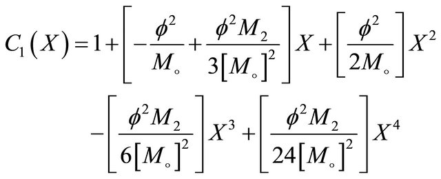
By solving the Equation (12), we can obtain the concentration of VOC for Andrews kinetics as follows,
 (22)
(22)
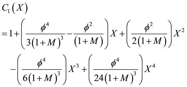
Solving the dimensionless form of Interactive model from Monod kinetics Equation (14), we get the concentration as,
 (23)
(23)
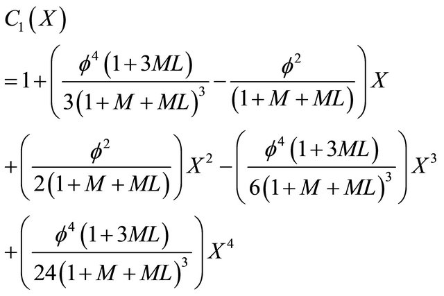
Solving the dimensionless form of Interactive model from Andrews kinetics Equation (16), we get the concentration as,
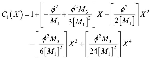 (24)
(24)
where
 ,
,
 ,
,
 , and
, and
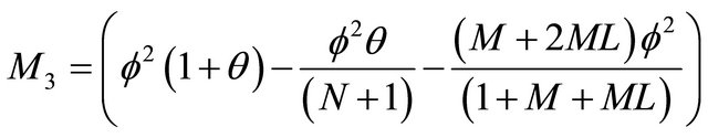 .
.
4. Effectiveness Factor
The effectiveness factor is defined as the ratio of actual rate of reaction to the rate of reaction that would result if the entire biofilm was exposed to the concentration at the gas/biofilm interface. The effectiveness factor of various kinetics are as follows:
Monod kinetics
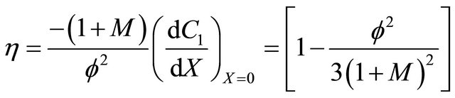 (25)
(25)
Andrews kinetics
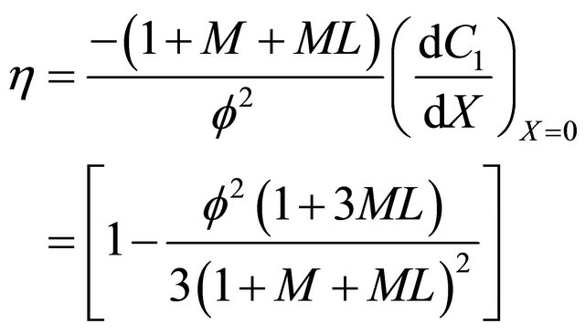 (26)
(26)
Interactive model from Monod kinetics
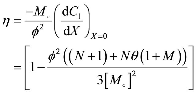 (27)
(27)
Interactive model from Andrews kinetics
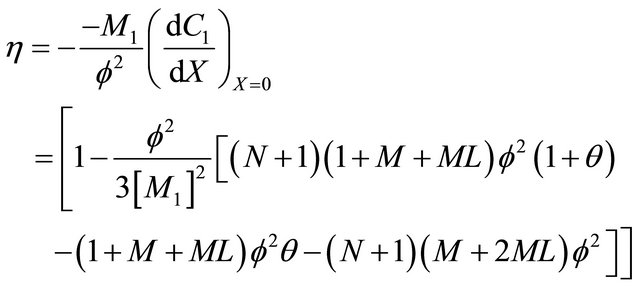 (28)
(28)
5. Numerical Simulation
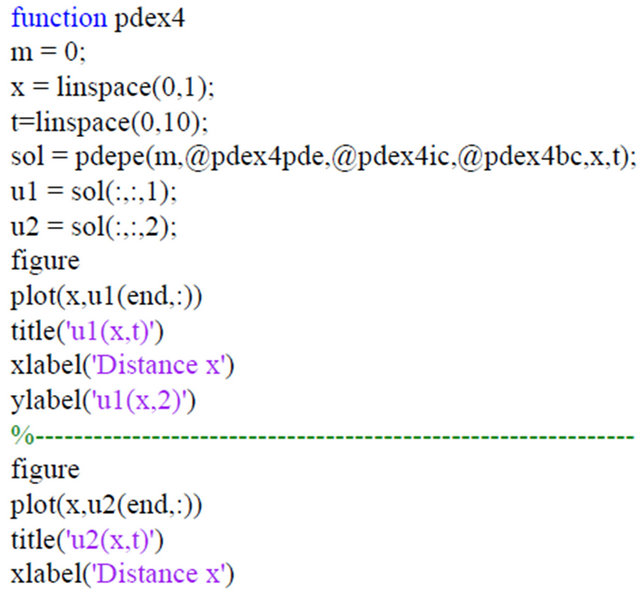
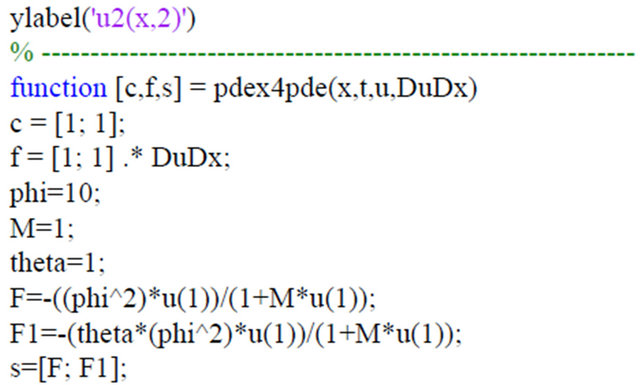
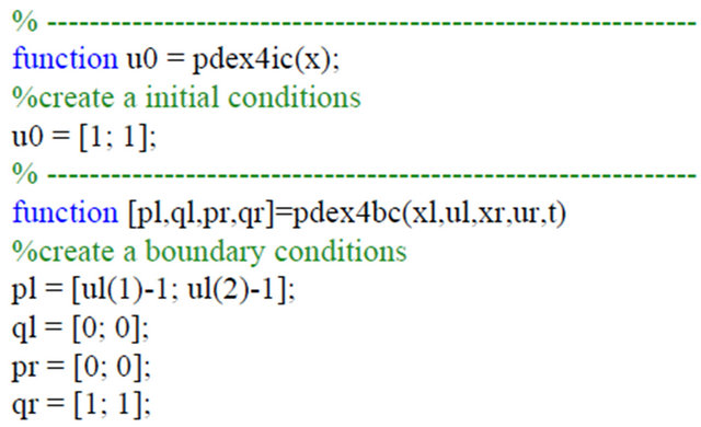
The dimensionless form of Equations (10)-(17) corresponding to the boundary conditions (18) and (19) were solved by numerical methods. We have used pdex4 to solve these equations (Pdex4 in MATLAB is a function to solve the initial-boundary value problems of differential equations. Matlab program to find the numerical solution of Equations (10) and (11) is given in the Appendix B. The numerical solution is compared with our analytical results and is shown in Figures 2-9. A satisfactory agreement is noticed for various values of the Thiele modulus and possible small values of reaction/ diffusion parameters.
6. Discussion
Equations (21)-(24) represents the new analytical expressions of the concentration of VOC for Monoid, Andrews, Interactive Monoid and Interactive Andrews kinetics for all values of the parameter. Using the relation (Equation (20)), we can also obtain the concentration of oxygen  for all the kinetics. Zarook et al. [17] obtained the
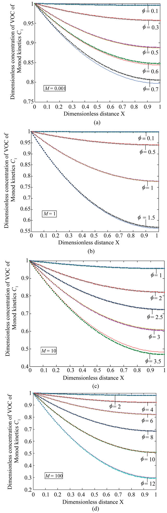
Figure 2. The dimensionless concentration C1 versus dimensionless distance X for various values of Thiele modulus f and M using Equation (21).
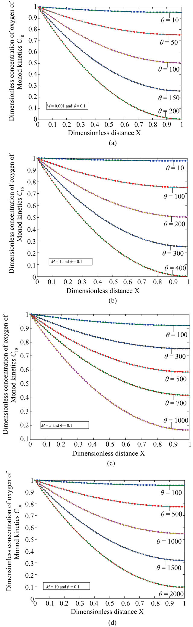
Figure 3. The dimensionless concentration C10 versus dimensionless distance X for various values of dimensionless quantity θ, M and f using Equation (20).
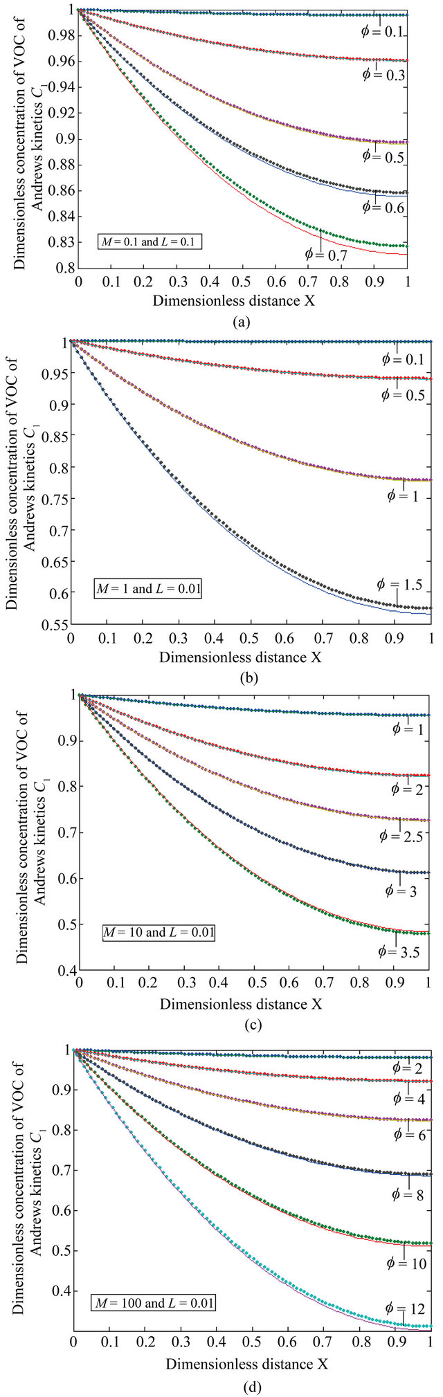
Figure 4. The dimensionless concentration C1 versus dimensionless distance X for various values of Thiele modulus f, M and L using Equation (22).
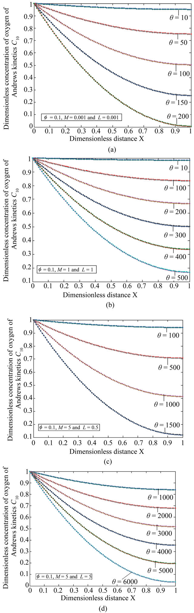
Figure 5. The dimensionless concentration C10 versus dimensionless distance X for various values of dimensionless quantity θ, M, L and f using Equation (20).
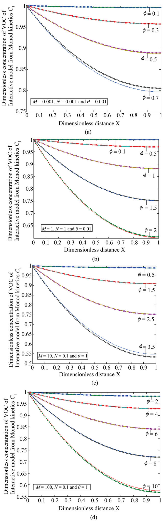
Figure 6. The dimensionless concentration C1 versus dimensionless distance X for various values of Thiele modulus f, M, N and θ using Equation (23).
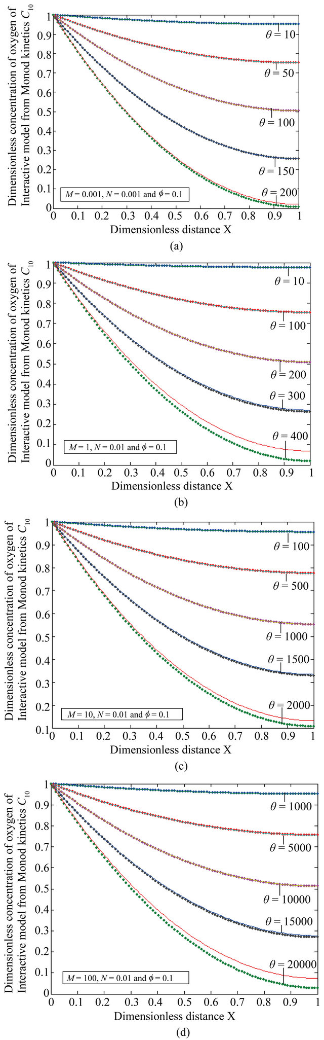
Figure 7. The dimensionless concentration C10 versus dimensionless distance X for various values of dimensionless quantity θ, M, L and f using Equation (20).
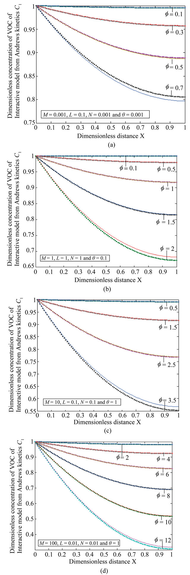
Figure 8. The dimensionless concentration C1 versus dimensionless distance X for various values of Thiele modulus f, M, L, N and θ using Equation (24).
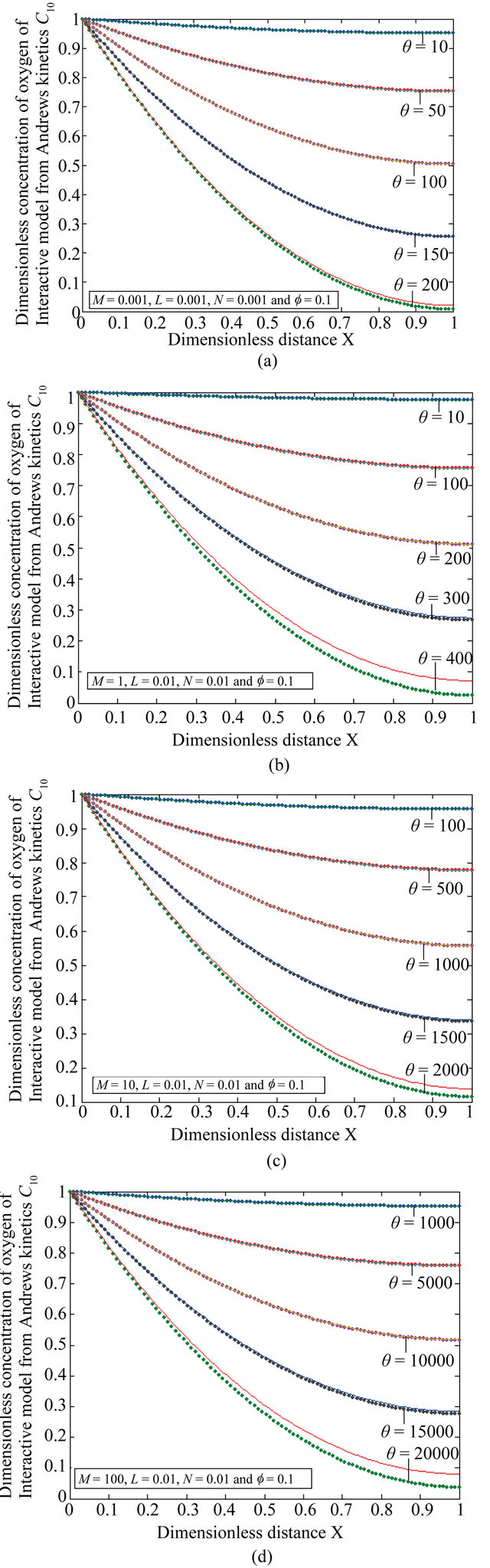
Figure 9. The dimensionless concentration C10 versus dimensionless distance X for various values of dimensionless quantity θ, M, L, N and f using Equation (20).
analytical expressions of concentration of VOC and oxygen only for the limiting cases (Zero kinetics and First-order kinetics). Concentration of VOC  and oxygen
  depends upon the value of parameters
 ,
,  , L, N and
 .
.
6.1. The Thiele Modulus
The Thiele module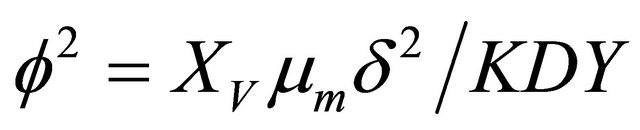 , essentially compares biodegradation rate
  with diffusion rate
 . We observe the rise and downfall of concentration profiles in two cases. 1) If Thiele modulus is small
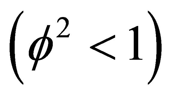 , then enzyme kinetics predominate. The overall kinetics is governed by the total amount of active enzyme; 2) The response is under diffusion control, if the Thiele module is large
 , which is observed at high catalytic activity and active membrane thickness or at low reaction kinetic constant
 ![]() or diffusion coefficient values
or diffusion coefficient values .
.
6.2. Monod Kinetics
Equation (21) represents the concentration of VOC for Monod kinetics in the biofilm.
Figures 2(a)-(d) is the plot of dimensionless concentration  versus dimensionless distance X for various values of Thiele modulus
  and the dimensionless quantity M using Equation (21). From this Figure it is inferred that, the concentration of VOC, at
 , increase when the value of
  or bio-filter thickness decreases. Also the concentration is uniform when
  and all values of
 .
.
Figures 3(a)-(d) is the plot of dimensionless concentration  for various values of dimensionless quantity
 ,
, and the Thiele modulus
 . From this figure it is observed that the concentration of oxygen is decreases when
  increases.
6.3. Andrews Kinetics
Equation (22) is the concentration of VOC for Andrews-type kinetics.
Figures 4(a)-(d) is the plot of dimensionless concentration  versus dimensionless distance X for various values of dimensionless parameters. From this figure, it is noted that the concentration of VOC decreases when
 ,
, ![]() ,
,  increases.
Figures 5(a)-(d) represents the dimensionless concentration  for various values of dimensionless quantity
 ,
,  ,
, ![]() and
and .
.
6.4. Interactive Monod Kinetics
Equation (23) represents the concentration of VOC of Interactive model from Monod kinetics.
Figures 6(a)-(d) is the dimensionless concentration  versus dimensionless distance X for various values
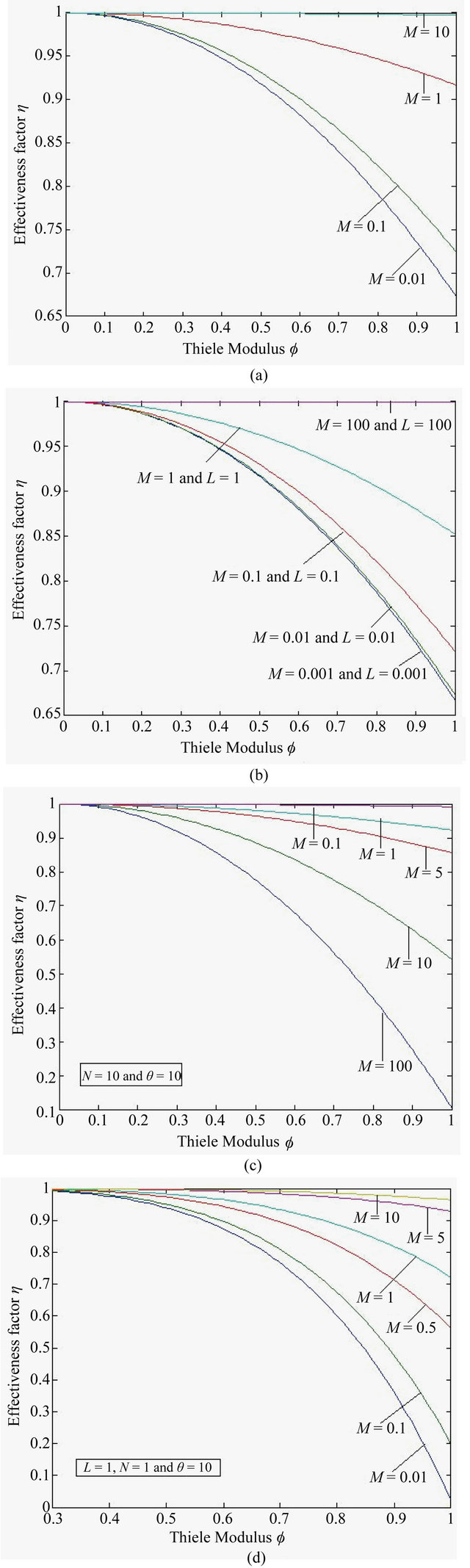
Figure 10. Effectiveness factor η versus the Thiele modulus f using the Equations (25)-(28) respectively.
of parameters using Equation (23). From this Figure it is noted that, the concentration of  is uniform when
 . Also
  decreases when θ increases whereas the Figures 7(a)-(d) for the dimensionless concentration
  for various values of dimensionless quantity
 ,
,  ,
,  and
and . From this figure it is inferred that the concentration of VOC
  is equal to one when
  for all values of parameters.
6.5. Interactive Andrews Kinetics
Equation (24) is the concentration of VOC of Interactive model from Andrews kinetics.
Figures 8(a)-(d) is the dimensionless concentration  versus dimensionless distance X for various values of Thiele modulus
 ,
,  ,
, ![]() ,
,  and
and  using Equation (24).
Figures 9(a)-(d) is the dimensionless concentration  for various values of dimensionless parameters. From this figure it is inferred that the concentration of VOC
  is constant when bio-filter thickness
  decreases.
6.6. Effectiveness Factor
Figures 10(a)-(d) represent the effectiveness factor  versus the Thiele modulus
  using Equations (25)-(28). From this figure it is observed that the effectiveness factor = 1 when
  for all mechanisms. Also the effectiveness factor decreases when
  increases and the values of parameters
  and
and ![]() decreases.
decreases.
7. Conclusion
The non-linear differential equations in biofilter models have been solved analytically for various kinetics using the Adomian decomposition method. Analytical expression of concentration of VOC and oxygen and corresponding effectiveness factor have been obtained for Monoid, Andrews, Interactive Monoid and Andrews kinetics and for all values of parameters. These analytical reactions very much useful for designing or scaling-up of biofilters.
8. Acknowledgements
This work was supported by the University Grants Commission (F. No. 39-58/2010(SR)), New Delhi, India and Council of Scientific and Industrial Research (CSIR No.: 01(2442)/10/EMR-II), New Delhi, India. The authors are thankful to Dr. R. Murali, The Principal, The Madura College, Madurai and The Secretary, Madura College Board, Madurai for their encouragement.
REFERENCES
- S. P. P Ottengraf, H. J. Rehm and G. Reed, Eds., “Exhaust Gas Purification,” Biotechnology, Vol. 8, 1986, pp. 425-452.
- S. P. P. Ottengraf and A. H. C. Van den Oever, “Kinetics of Organic Compound Removal from Waste Gases with a Biological Filter,” Biotechnology and Bioengineering, Vol. 25, No. 12, 1983, pp. 3089-3102. doi:10.1002/bit.260251222
- S. M. Zarook, B. C. Baltzis, Y.-S. Oh and R. Bartha, “Biofiltration of Methanol Vapor,” Biotechnology and Bioengineering, Vol. 41, No. 5, 1993, pp. 512-524. doi:10.1002/bit.260410503
- E. R. Allen and S. Phatak, “Control of Organosulfur Ompound Emissions Using Biofiltration. Methyl Mercaptan,” Proceedings of the 86th, Air and Waste Management Association Annual Meeting and Exhibition, Denver, 13-18 June 1993.
- M. A. Deshusses and I. J. Dunn, “Modeling Experiments on the Kinetics of Mixed-Solvent Removal from Waste Gas in a Biofilter,” Proceedings of the 6th European Congress in Iotechnology, Florence, 13-17 June 1993.
- S. M. Zarook and B. C. Baltzls, “Biofiltration of Toluene Vapour under Steady State and Transient Conditions,” Chemical Engineering Science, Vol. 49, 1994, pp. 4347- 4360. doi:10.1016/S0009-2509(05)80026-0
- S. P. P. Ottengraf, R. M. M. Diks, “Biotechniques for Air Pollution Abatement and Odor Control Policies,” Process Technology of Biotechniques, Elsevier Science, New York, 1992, pp. 17-31.
- C. Van Lith, S. L. David and R. Marsh, “Design Criteria for Biofilters,” Transactions of the Institution of Chemical Engineers, Vol. 68, 1990, pp. 127-132.
- D. S. Hodge and J. S. Devinny, “Modeling Removal of Air Contaminants by Biofiltration,” Journal of Environmental Engineering, Vol. 121, No. 1, 1995, pp. 21-32. doi:10.1061/(ASCE)0733-9372(1995)121:1(21)
- M. A. Deshusses, G. Hamer and I. J. Dunn, “Behavior of Biofilters for Waste Air Biotreatment,” Journal of Environmental Science Technology, Vol. 29, No. 4, 1995, pp. 1048-1068. doi:10.1021/es00004a027
- E. Morgenroth, E. D. Schroeder, D. P. Y. Chang and K. M. Scow, “Modeling of a Compost Biofilter Incorporating Microbial Growth,” American Society of Civil Engineers, 1995, pp. 473-480.
- R. S. Cherry and D. N. Thompson, “The Shift from Growth to Nutrient limited Maintenance Kinetics during acclimation of a Biofilter,” Journal of Biotechnology Bioengineering, Vol. 56, No. 3, 1997, pp. 330-339. doi:10.1002/(SICI)1097-0290(19971105)56:3<330::AID-BIT11>3.0.CO;2-K
- S. M. Zarook, A. A. Shaikh and Z. Ansar, “Development, Experimental Validation and Dynamic Analysis of a General Transient Biofilter Model,” Journal of Chemical Engineering Science, Vol. 529, No. 5, 1997, pp. 759-773. doi:10.1016/S0009-2509(96)00428-9
- S. M. Zarook and A. A. Shaikh, “Analysis and Comparison of Biofilter Models,” Chemical Engineering Journal, Vol. 65, No. 1, 1997, pp. 55-61. doi:10.1016/S1385-8947(96)03101-4
- A. Coely, Eds., et al., “Backlund and Darboux Transformation,” American Mathematical Society, Providence, 2001.
- M. Wadati, H. Sanuki and K. Konno, “Relationships among Inverse Method, Bäcklund Transformation and an Infinite Number of Conservation Laws,” Progress of the Theoretical Physics, Vol. 53, No. 2, 1975, pp. 419-436. doi:10.1143/PTP.53.419
- C. S. Gardener, J. M. Green, M. D. Kruskal and R. M. Miura, “Method for Solving the Korteweg-de Vries Equation,” Physical Review Letters, Vol. 19, No. 19, 1967, pp. 1095-1097. doi:10.1103/PhysRevLett.19.1095
- R. Hirota, “Exact Solution of the Korteweg-De Vries Equation for Multiple Collisions of Solitons,” Physical Review Letters, Vol. 27, No. 18, 1971, pp. 1192-1194. doi:10.1103/PhysRevLett.27.1192
- W. Malfliet, “Solitary Wave Solutions of Nonlinear Wave Equations Solitons,” American Journal of Physics, Vol. 60, No. 7, 1992, p. 650. doi:10.1119/1.17120
- J. H. He, “Approximate Analyticalsolution for Seepage Flow with Fractionalderivatives in Porous Media,” American Computer Methods in Applied Mechanics and Engineering, Vol. 167, No. 1-2, 1998, pp. 57-68. doi:10.1016/S0045-7825(98)00108-X
- J. H. He, “Chaos Solitons Fractals,” Applied Mathematics and Computation, Vol. 26, No. 3, 2005, p. 695.
- J. H. He, “Homotopy Perturbation Method for Solving Boundary Value Problems,” Physics Letters A, Vol. 350, No. 1-2, 2006, pp. 87-88. doi:10.1016/j.physleta.2005.10.005
- J. H. He, “A Simple Perturbation Approach to Blasius Equation,” Applied Mathematics and Computation, Vol. 140, No. 2-3, 2003, pp. 217-222. doi:10.1016/S0096-3003(02)00189-3
- D. D. Ganji and M. Rafei, “Solitary Wave Solutions for a Generalized Hirota-Satsuma Coupled KdV Equation by Homotopy Perturbation Method,” Physics Letters A, Vol. 356, No. 2, 2006, pp. 131-137. doi:10.1016/j.physleta.2006.03.039
- P. D. Ariel, “Homotopy Perturbation Method and the Natural Convection Flow of a Third Grade Fluid through a Circular Tube,” Nonlinear Science Letters A, Vol. 1, 2010, pp. 43-52.
- B. Jang, “Two-Point Boundary Value Problems by the Extended Adomian Decomposition Method,” Journal of Computational and Applied Mathematics, Vol. 219, No. 1, 2008, pp. 253-262. doi:10.1016/j.cam.2007.07.036
- G. Adomian, “Solutions of Nonlinear PDE,” Applied Mathematics, Vol. 11, No. 3, 1998, pp. 121-123.
- G. Adomian, “A Global Method for Solution of Complex Systems,” Mathematical Modelling, Vol. 5, No. 4, 1984, pp. 251-263. doi:10.1016/0270-0255(84)90004-6
- G. Adomian, “Stochastic Nonlinear Modeling of Fluctuations in a Nuclear Reactor—A New Approach,” Annals of Nuclear Energy, Vol. 8, No. 7, 1981, pp. 329-330. doi:10.1016/0306-4549(81)90053-0
- A. Saufyane and M. Boulmalf, “Solution of Linear and Nonlinear Parabolic Equations by the Decomposition Method,” Applied Mathematics and Computation, Vol. 162, No. 2, 2005, pp. 687-693. doi:10.1016/j.amc.2004.01.005
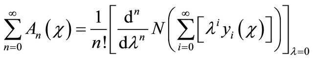
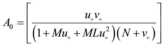
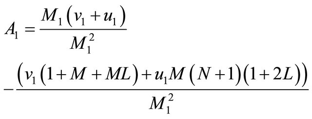
Appendix A
Analytical Solution of Non-Linear (Equation (16)) Using The Adomian Decomposition Method In the operator form, Equation (16) becomes
 (B1)
(B1)
where
and
 (B2)
(B2)
Applying  to both sides of (B1) yields
 (B3)
(B3)
where a and b are constants of integration. To solve (B3) by the Adomian method, we get
 (B4)
(B4)
 (B5)
(B5)
In view of the Equations (B4)-(B5), Equation (B3) gives
 (B6)
(B6)
we identify the zeroth component as
 (B7)
(B7)
and the remaining components as the recurrence relation,
![]() (B8)
(B8)
where  are the Adomian polynomials that represent the non-linear term in (B8).
 (B9)
(B9)
Using (B9) we can find the first few  as follows:
 (B10)
(B10)
 (B11)
(B11)
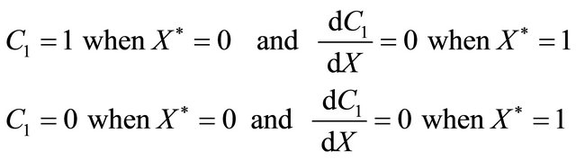
The remaining polynomials can be generated easily. The corresponding boundary condition becomes
 (B12)
(B12)
Substitution of (B10) and (B11) in (B8) and operating with  in conjunction with the boundary conditions (B12) in each case separately, we obtain
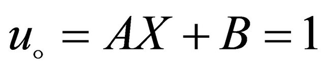 (B13)
(B13)
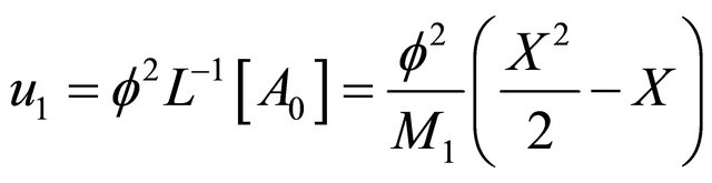 (B14)
(B14)
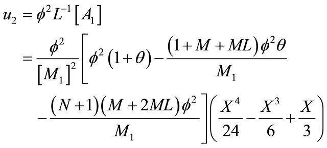 (B15)
(B15)
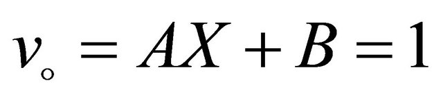 (B16)
(B16)
 (B17)
(B17)
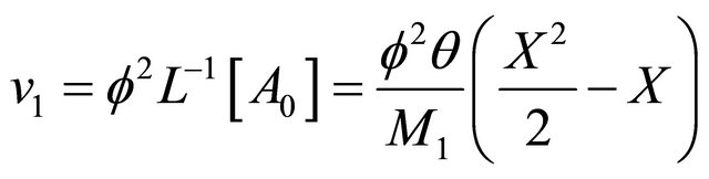
Substituting the Equations (B13)-(B15) in
 (B18)
(B18)
we can obtain the Equation (24) in the text. Similarly, applying the above same procedure, we obtain the Equations (21)-(23).
Appendix B
Matlab/Scilab program to find the numerical solution of the Equations (10)-(11).
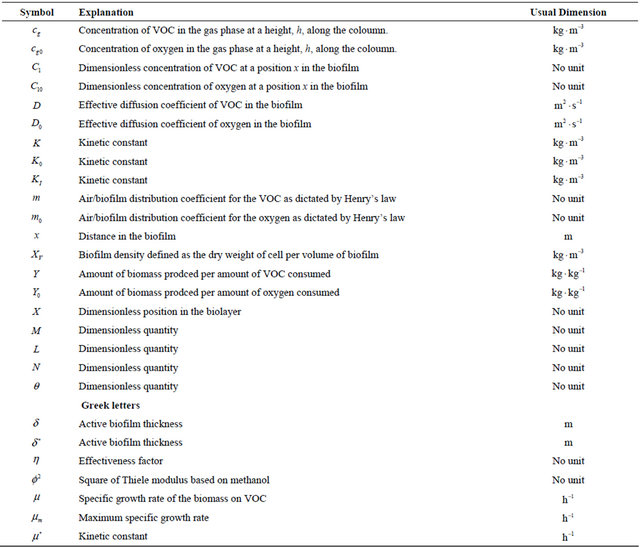
Nomenclature and Units
NOTES
*Corresponding author.