Applied Mathematics
Vol. 3 No. 1 (2012) , Article ID: 16768 , 7 pages DOI:10.4236/am.2012.31008
Lp-Estimations of Vector Fields in Unbounded Domains
Department of Mechanics and Mathematics, N. I. Lobachevsky State University of Nizhny Novgorod, Nizhny Novgorod, Russia
Email: Artem.Zhidkov@gmail.com
Received November 15, 2011; revised December 15, 2011; accepted December 23, 2011
Keywords: Estimations; Scalar Product; Vector Field; Functional Spaces; Maxwell Equations; Solvability; Inhomogeneous Domains
ABSTRACT
Some new estimations of scalar products of vector fields in unbounded domains are investigated. Lp-estimations for the vector fields were proved in special weighted functional spaces. The paper generalizes our earlier results for bounded domains. Estimations for scalar products make it possible to investigate wide classes of mathematical physics problems in physically inhomogeneous domains. Such estimations allow studying issues of correctness for problems with non-smooth coefficients. The paper analyses solvability of stationary set of Maxwell equations in inhomogeneous unbounded domains based on the proved Lp-estimations.
1. Introduction
The estimations of scalar products of vector fields and their norms play a significant role in proving the solvability of mathematical physics problems. Many researches are devoted to the study of estimates of the norms of vector functions in different functional spaces [1-4]. But in the most cases such estimations require the homogeneous areas when their parameters don’t depend on space coordinates [5,6].
For inhomogeneous areas we suggest using estimations of scalar products of vector fields for the mathematical physics problems. In the publications [7-10] some Lp-estimations of scalar product of vector fields in the limited areas were obtained and was investigated the possibility of their application to study the solvability of different problems of electromagnetic theory.
It is natural to study problem formulations in non-homogeneous unbounded domains for most problems of mathematical physics. In the publications [11,12] we proved L2-estimations of scalar products of vector fields in unlimited areas.
The paper is dedicated to solvability of a stationary set of Maxwell equations in the whole  space, based on the proved Lp-estimations of scalar product in the weighted functional spaces.
2. Main Functional Spaces
Let  be an open subset of
  space (particularly
 ).
).
Let  be a Banach space of functions
 , summable with power
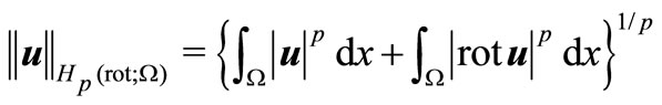
 , where a norm is
Let  be a Banach space of vector-functions
 ,
,
where  (
( ), with a norm
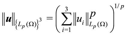 .
.
Let  and
and  be Banach spaces
with norms
 respectively.
We denote by  and
and  the closures of the set of test vector-functions in
  and
and , respectively.
The following estimates for scalar products of vector fields in the bounded star-shaped domain  with the regular boundary were obtaned in [8,9,11].
Lemma 2.1. Let ,
, . There exists a constant
 , that for any
 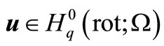 and
and 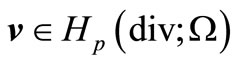
Lemma 2.2. Let ,
, . There exists a constant
 , that for any
  ,
, 
Lemma 2.3. Let ,
, . There exists a constant
 , that for any
  and
and 
The main result of this paper is a proof of similar estimates for .
.
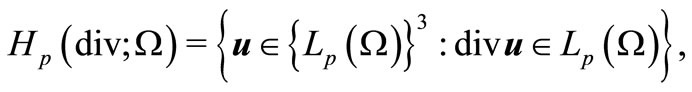
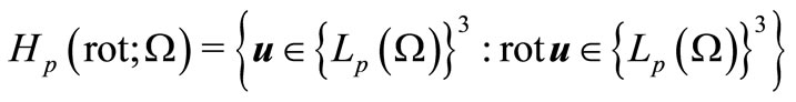
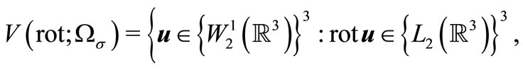
Let . For each
  and
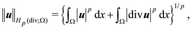
and  we define Banach spaces of vector-functions:
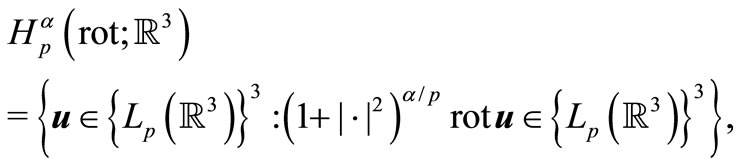
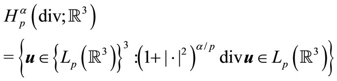
with the corresponding norms
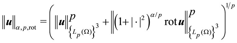 ,
,
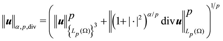 .
.
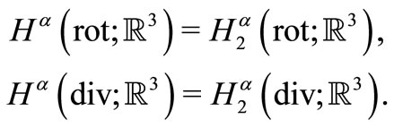
For  [12] these spaces are defined as:
3. Estimations of Scalar Products
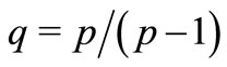
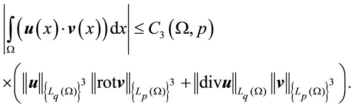
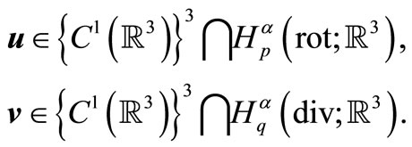
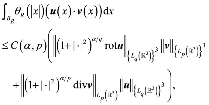
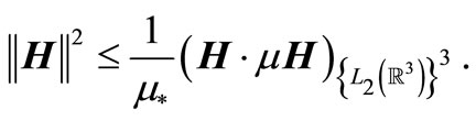
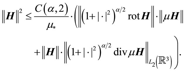
The main result of the current article is Theorem 3.1. Let ,
,  ,
,  ,
, . Then there exists a positive constant
  , which does not depend on vector-functions
 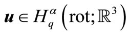 and
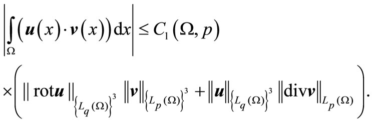
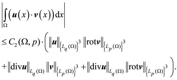
and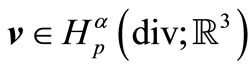 , and the inequality
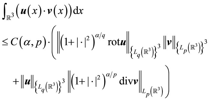 (1)
(1)
is correct.
In proving Theorem 3.1 the following statement is used.
Lemma 3.2 [7]. Let  be an open set in
  (particularly,
 ) star-shaped on
 . Then the following identities are true for all
  and each function
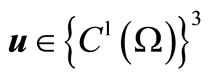
 (2)
(2)
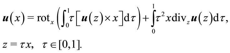 (3)
(3)
Let ,
,  ,
, . Then the identities (2) and (3) are equivalent to
 (4)
(4)
 (5)
(5)
Proof (Theorem 3.1). Let . Let
. Let  and
and  be smooth vector-functions on
Let  denote a closed solid sphere with radius
  centered at the origin and with the boundary
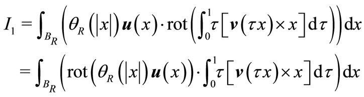
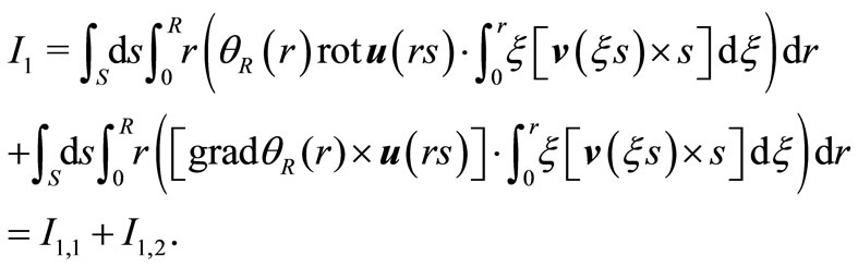
 . Consider the integral
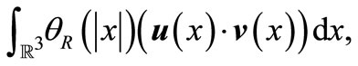 (6)
(6)
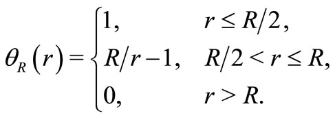
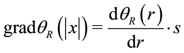
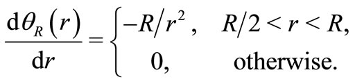
where  is a function of scalar argument
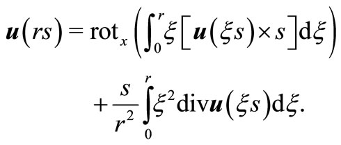
We use the representation (3) for the vector-function  in the integral (6)
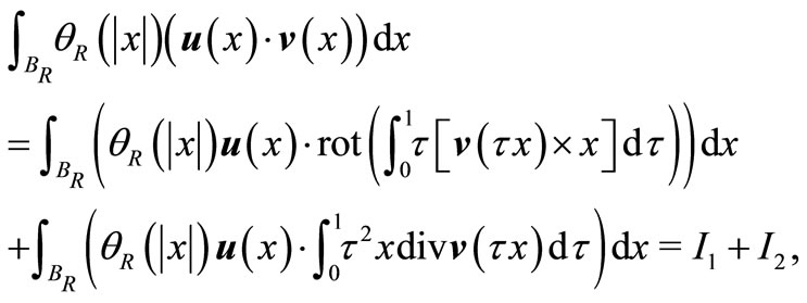
For the first of resulting integrals ( ) we use a vector field relation
and then we invoke the Gauss-Ostrogradsky theorem and use the fact that  when
when . So
. So
or passing to spherical coordinates the operator 
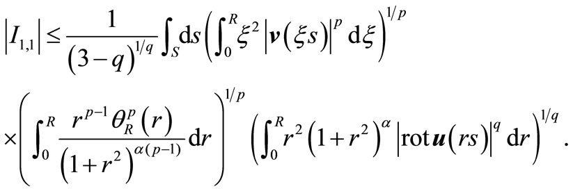
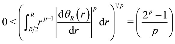
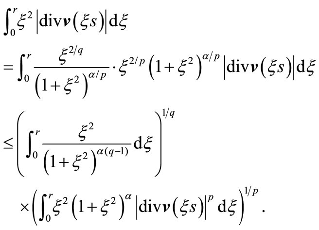
We estimate the first integral. Applying Hölder’s inequality to 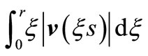 we get
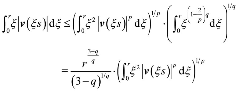
then
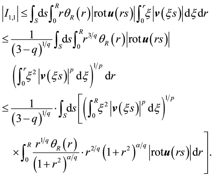
Applying Hölder’s inequality to the second inner integral, we have:
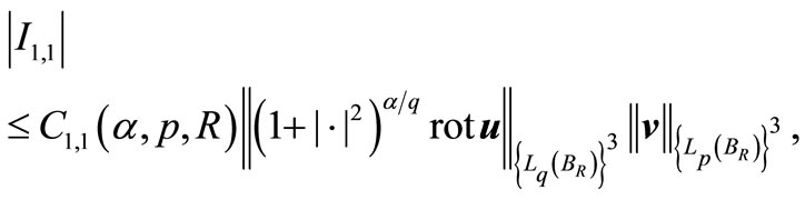
We can write the estimation as

It is obvious that if  an expression
  , then
Let us estimate the integral . It is evident the the
 , where
Applying Hölder’s inequality several times, we get
The following estimation is obvious
Hense
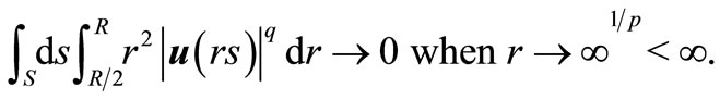
then  when
when .
.
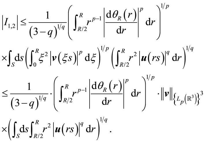
Next we construct an estimation for integral . We apply Hölder’s inequality to
 .
.
So, we get an estimation for :
:
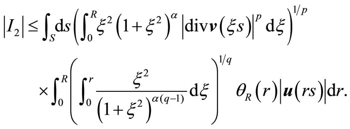
We use Hölder’s inequality for the second integral again.
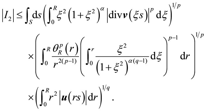
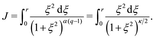
Let’s estimate the following integral
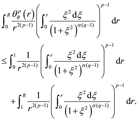
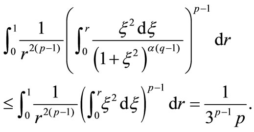
Denote 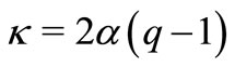 and consider
When  (i.e.
(i.e.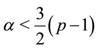 ), then
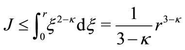
and, respectively
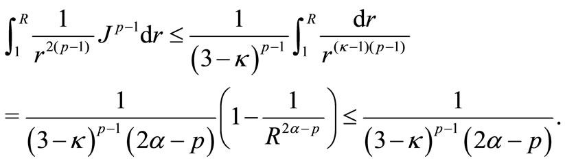
If  we get
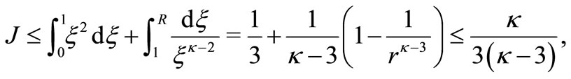
At last, when , then


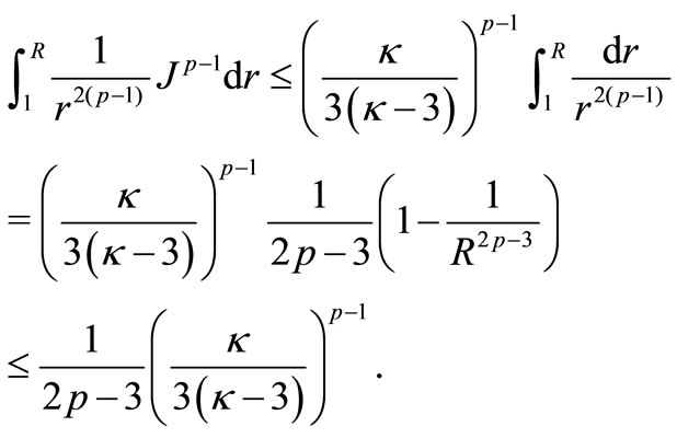
Thus, we obtain
and therefore

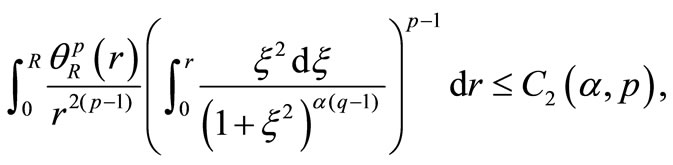
Bringing together the constructed estimates, we derive the following inequality for integral (6)
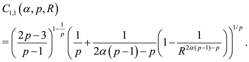
where
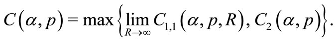
Going to the limit for  in the last inequality, we will obtain estimation (1).
Note, that for  the theorem may be proved similarly using the Equivalence (2).
4. Discussion of the Stationary Problem of Electromagnetic Theory
As an example of using the estimations proved in Section 3, we will consider a problem of determining the magnetic field stretch  in the whole
  space with a bounded conducting subdomain.
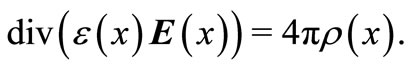
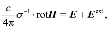
Stationary electromagnetic field is described by the set of stationary Maxwell’s equations
 (7)
(7)
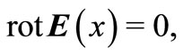 (8)
(8)
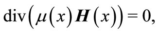 (9)
(9)
 (10)
(10)
Here . The conductivity of the atmosphere is denoted as
 . Let
. Let  denotes a bounded open star-shaped subset of
  defined by conditions
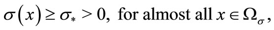 (11)
(11)
 (12)
(12)
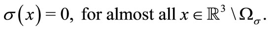
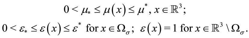
Functions 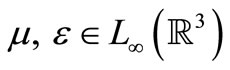 are permeability and permittivity. They satisfy the following conditions
The  is a vector-function of the external electromotive force, which is asumed given and satisfying the condition
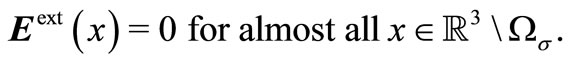
Function  equals zero for almost all
  .
.
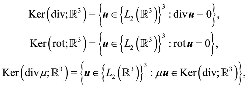
We introduce the necessary functional spaces
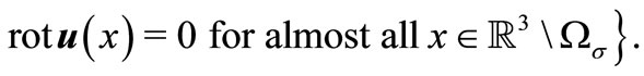
Denote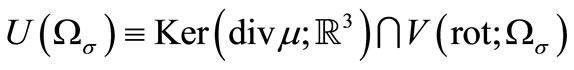 . It is readily proved that this functional space will be Hilbert space relatively to scalar product

We name the solution of the Problem (7)-(10) the functions ,
,  and
and  satisfying condition
  for almost all
 .
.
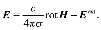
The validity of (10) implies the distibution  for all
  defined by the formula
 (13)
(13)
Equation (7) in conducting subdomain will be
and in nonconducting subdomain ( ) it becomes an identity.
Multiplying the last equation by ,
,  , integrating along
 , and using
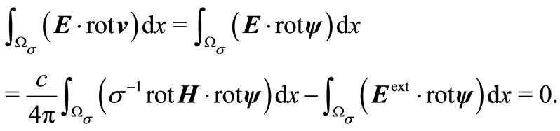
  or
or
 .
.
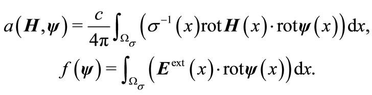
It becomes obvious that the problem of determining the stationary magnetic field can be formulated as follows:
Determine vector-function  satisfying the integral identity
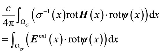 (14)
(14)
for all functions .
.
We need the following statement to prove the theorem of solvability (Theorem 4.2) for the Problem (14).
Lemma 4.1 (Lax-Milgram [13]). Let  be a Hilbert space over the field of real numbers. Let
  be a symmetric bilinear bounded coercive form,
 —linear bounded functional. Then there exists a unique element
  satisfying the equality

for all .
.
Theorem 4.2 (Solvability of the Problem (14)). Let
 satisfy (11), (12),
  and
and
 for almost all
 . Then the solution
  of the generalized Problem (14) exists and is unique.
Proof. Let’s verify the conditions of the Lax-Milgram lemma.
Let us denote
Obviously,  is a bilinear and symmetric form. The finiteness is easily proved by condition (11):
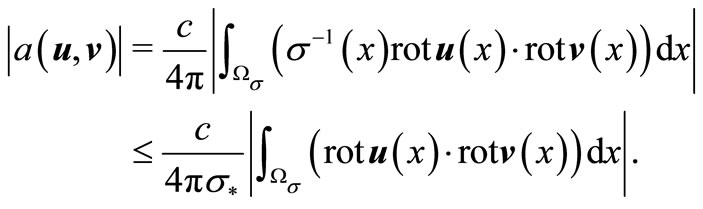
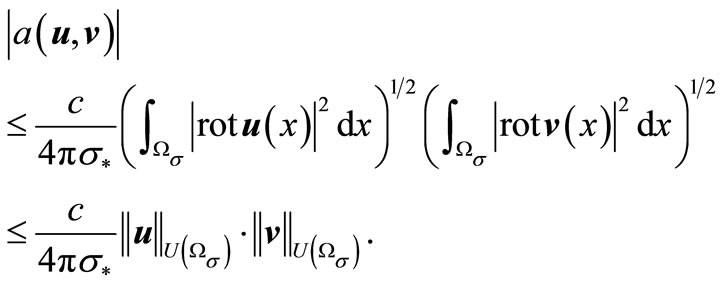
Using the Cauchy-Bunyakovsky-Schwarz inequality, we obtain
Let’s show coercivity of the form .
.
Whereas  thus
thus 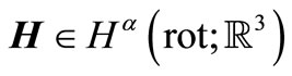 for each
 , i.e. the vector-function
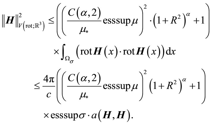
  satisfies estimation
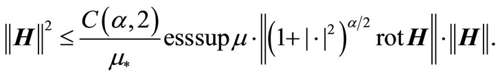
The following notation is used . Let’s use Estimation (1)
Since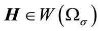 , the last summand is zero. Then using the Hölder’s inequality, we obtain
Hense
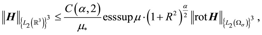
where . The estimates show the coercivity of the bilinear form, because
Now we verify the conditions for functional . The linearity is obvious. Let’s show the finiteness using the Cauchy-Bunyakovsky-Schwarz inequality
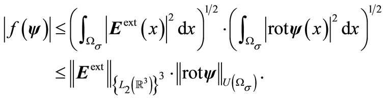
Thus, all the constraints of the Lax-Milgram lemma are satisfied, and the solution of the Problem (14) exists and is unique.
Remark. The solvability of the studied problem is also true when  is a positive-definite tensor. The scheme of the proof is similar to Theorem 4.2.
Let  satifies relation (14) for all
 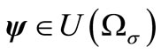 . Let’s show that other indefinite functions will be defined in
  from equaitons (7)-(10) as values depending on
 .
.
We determine function  in the conductivity area by equality
Let . Let’s extend
  by zero in
 . According to the Lax-Milgram lemma there is the unique function
 , which for each
  satisfies the equality
Then  and as
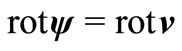 , then
 . Therefore we obtain that
This shows that .
.
The function  is defined by relation (13) as shown above.
5. Conclusion
The paper was devoted to the proof of Lp-estimation of vector fields in weighted functional spaces. Also we discussed a solvability of the problem of determinig the magnetic field stretch in the whole  space. The proof of solvability is based on the proved estimation.
6. Acknowledgements
This work was supported by Analytical Departmental Program “Highschool scientific potential growth” (2009- 2011) Russian Ministry of Education and Science (reg. no. 2.1.1/3927), Federal Target Program “Scientific and Scientific-Pedagogical Personnel of Innovative Russia” (2009-2013) (project NK-13P-13) and RFBR Grant (project 09-01-97019-r_povolzhie_a).
REFERENCES
- E. Byhovskii and N. Smirnov, “Orthogonal Decomposition of the space of vector functions square-summable on a given domain, and the operators of vector analysis,” (Russian) Trudy Matematicheskogo Instituta Steklov, Vol. 59, 1960, pp. 5-36.
- G. Duvaut and J. Lions, “Inequalities on Mechanics and Physics,” Springer-Verlag, Berlin, 1976. doi:10.1007/978-3-642-66165-5
- R. Temam, “Navier-Stokes Equations: Theory and Numerical Analysis,” North-Holland Publishing Company, Amsterdam, 1977.
- H. Weil, “The method of orthogonal Projection in potential theory,” Duke Mathematics Journal, Vol. 7, No. 1, 1940, pp. 411-444. doi:10.1215/S0012-7094-40-00725-6
- V. Girault and P.-A. Raviart, “Finite Element Approximation of the Navier-Stokes Equations,” Springer-Verlag, New-York, 1979.
- V. Maslennikova, “Lp estimates, and the asymptotics at t→∞ of the solution of the Cauchy problem for a Sobolev system,” (Russian) Trudy Matematicheskogo Instituta Steklov, Vol. 103, 1968, pp. 117-141.
- A. Kalinin, “Some estimations in the theory of vector fields,” (Russian) Vestnik UNN Series Mathematical Modeling and Optimal Control, Nizhny Novgorod, No. 20, 1997, pp. 32-38.
- A. Kalinin and A. Kalinkina, “Estimates of vector fields and stationary set of Maxwell equations,” (Russian) Vestnik UNN Series Mathematical Modeling and Optimal Control, No. 1, 2002, pp. 95-107.
- A. Kalinin and A. Kalinkina, “Lp-estimates for Vector fields,” Russian Mathematics (Izvestiya Uchebnykh Zavedenii Matematika), Vol. 48, No. 3, 2004, pp. 23-31.
- A. Kalinin, S. Morozov, “Stationary problems for the set of Maxwell equations in heterogeneous areas,” (Russian) Vestnik UNN Series Mathematical Modeling and Optimal Control, No. 20, 1997, pp. 24-31.
- A. Kalinin, “Estimations of scalar products for vector fields and their application in some problems of mathematical physics,” (Russian) Izvestiya of Institution of Mathematics and Infomatics UdSU, Vol. 3, No. 37, 2006, pp. 55-56.
- A. Zhidkov, “Estimates of the scalar products of vector fields in unbounded regions,” (Russian) Vestnik UNN, Nizhny Novgorod, No. 1, 2007, pp. 162-166.
- P. Lax and A. Milgram, “Parabolic Equations,” Annals of Mathematics Studies, Vol. 33, 1954, pp. 167-190.