Modern Economy
Vol.5 No.1(2014), Article ID:42328,4 pages DOI:10.4236/me.2014.51008
Environmental Kuznets Curve for Water Pollution: The Case of Border Countries
Department of Economics, Indiana University of Pennsylvania, Indiana, USA
Email: Alexi.Thompson@iup.edu
Copyright © 2014 Alexi Thompson. This is an open access article distributed under the Creative Commons Attribution License, which permits unrestricted use, distribution, and reproduction in any medium, provided the original work is properly cited. In accordance of the Creative Commons Attribution License all Copyrights © 2014 are reserved for SCIRP and the owner of the intellectual property Alexi Thompson. All Copyright © 2014 are guarded by law and by SCIRP as a guardian.
Received October 16, 2013; revised November 16, 2013; accepted November 23, 2013
KEYWORDS
Environmental Kuznets Curve; Water Pollution; Border Countries
ABSTRACT
This paper looks for evidence of an environmental Kuznets curve for water pollution in countries that share major rivers as their border. The data in this paper consist of a panel of 21 years and 30 countries, seven of which are border countries. The turning point for the border countries is much lower than that for the other subset. A t-test comparing group means for income and biochemical oxygen demand levels for both subsets finds no statistical difference for either variable, implying that countries sharing a river may be able to enforce environmental regulations more effectively than countries not sharing a river.
1. Introduction
This paper looks for an environmental Kuznet’s curve (EKC) for water pollution for countries that share a river as a border. The environmental Kuznet’s curve (EKC) hypothesis claims that pollution problems may be reduced by economic growth. The relationship between pollution and economic growth is described as an inverted ushape. The income level at which pollution degradation is maximized is known as the turning point. A number of explanations for this empirical result have been introduced including increased demand for environmental quality as income increases, and shifts in production from manufacturing to services.
Since initial work by Grossman and Kueger [1], many EKCs studies have been published on a number of differrent pollution indicators and methodologies with mixed results. Paudel, Zapata and Susanto [2] find evidence of an EKC for water pollution in Louisiana watershed data. Results from one-way fixed effects estimation showed EKC relationships for nitrogen, phosphorus, and dissolved oxygen with turning points of $11,572, $8508, and $9145. Lee, Chui, and Sun [3] do not find an EKC for water pollution for 97 countries for the period of 1980- 2001 in their EKC study on water pollution. The authors group countries into continental subgroups and find an EKC in America and Europe with turning points of $13,956 and $38,221. Granda, Perez, and Munoz [4] do not find an EKC for BOD on a panel data set of 46 countries for the years 1980-2000.
Typically, the turning point in water EKC is lower than that in air pollution [5]. In addition, water shortages are a major concern in many developing countries around the world. The underlying relationship between water pollution and economic growth is particularly important as poor countries grow richer.
This paper looks at countries that share a river as a common border. Shared rivers represent a common pool problem; without clearly defined property rights and environmental regulations between the two countries, the river divides may overuse this resource contributing to water pollution. Pooled mean group (PMG) estimation is used to estimate regressions on two subsets. One subset consists of 7 groups of countries whose border is formed by a major river. The other subset consists of other countries that do not have a major river forming a border with another country.
In the presence of a common pool problem, we may expect no EKC relationship between income and pollution in the border countries. Or, in the presence of an EKC relationship, there exists a higher turning point for the subset of countries whose border is formed by a major river (than for the other subset). Results indicate that an EKC exists for both subsets. Contrary to the suggestion of the common pool problem, the turning point for the border countries is much lower than for the other subset. A t-test comparing group means for income and biochemical oxygen demand levels for both subsets finds no statistical difference between the two subsets for either variable, implying that countries sharing a river are able to achieve river environmental regulations much more effectively than that countries not sharing a river.
2. Data
The data for this paper consists of a panel of 30 countries. Annual data runs from 1980 to 2000. The panel of 30 countries is divided into two subsections. The first subsection includes seven countries that share a river as a border with a neighboring country. These countries and the river lying on their border are listed in Table 1. Table 2 includes a list of other countries used in the study that comprise the second subset.
The water pollution indicator is biochemical oxygen demand (BOD). High BOD levels reduce oxygen contributing to death of aquatic life. BOD levels come from Earth Trends1 (2010). This variable is measured in kilo

Table 1. Border countries.

Table 2. Other countries.
grams per day and includes only industrial runoff, not agricultural runoff.
I assume the BOD levels reported by EarthTrends represent the actual pollution levels in the shared river. If BOD data was available for both countries in the border country subset, then BOD levels were averaged to represent the BOD level in the shared river. Income per capita comes from Penn World Tables (2009) with a base year of 2005. In the border country subset, the average of income per capita between the border countries was used in estimation.
The following figures plot BOD against income per capita. Country income per capita and BOD levels are averaged across countries within each subset from 1980 to 2000. The natural logarithm of the average of income per capita and BOD levels are depicted in the following figures. The first figure includes the subset of border countries and the second figure includes the subset of other countries. It is not evident that an EKC is evident in either subset. In the Figure 1, pollution levels do appear to eventually decrease as income per capita increases across countries over time. In Figure 2, there appears to be an S-shaped curve. That is, pollution initially decreases with respect to increases in income per capita, then increases as income per capita increases, before eventually decreasing again.
3. Method
Pooled mean group (PMG) estimation is used to estimate EKCs on two datasets; Model 1 is a subset of 7 pairs of

Figure 1. EKC in border countries.

Figure 2. EKC in other countries.
border countries and Model 2 includes other countries. Pooled mean group (PMG) estimation is used to estimate the EKC because Pesaran and Smith [6] show PMG estimates are consistent even in the presence of nonstationary variables. This dynamic panel estimation method is particularly suitable for EKC studies because it takes into account heterogeneity across countries.
The basic long run EKC relationship takes the form
 (1)
(1)
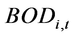
where  is biochemical oxygen demand measured in kilograms per day,
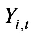
  is a country-specific intercept i denotes country and t denotes year. The pollution indicator is regressed on income
  and its squared term
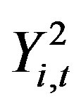
 . In the presence of an EKC,
  and
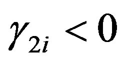
and  resulting in an inverted u-shaped EKC. With panel series spanning many years estimating Equation (1) could yield a spurious relationship between BOD and income Y.
The following autoregressive distributive lag ARDL model estimates short run EKC effects
 (2)
(2)
where the change in BOD ΔBOD is regressed on income, income squared, and lagged values of income, income squared, and BOD.
Finally, PMG estimation combines Equation (1) and Equation (2) in the following specification
 (3)
(3)
where 

PMG estimation allows short run coefficients to vary across countries but restricts long run coefficients to be same across countries. PMG estimation has been recently used in EKC studies [7,8]. All variables are in natural logarithms.
The Maddala and Wu (MW) [9] panel unit root test is used on the data because this panel unit root test does not require a balanced dataset. Income per capita is missing for the Czech Republic for four years making the panel unbalanced. The MW test has a null hypothesis of no panel unit root. Results from the MW tests are in Table 3. Stationary results are mixed. Income appears to have a unit root in Model 1, and BOD levels appear have a unit root in Model 2.
4. Results
Long run estimates from PMG estimation are in Table 4. The statistically significant negative error correction (EC) coefficients indicate a cointegrated relationship between pollution and income in Model 1 and Model 2.
An EKC is found in both subsets. The turning point in Model 1 is $3756 and for Model 2 $51,858. All the border countries in Model 1 have incomes higher than $3756 and none of the countries in the other subset have incomes above $51,858. The richest country in the Model 2 is Norway with income per capita of $34,000 in 2000.
In Model 2 it can be concluded that pollution is increasing in income. This is contrary to the common pool hypothesis and may be simply due to the countries that make up each subset. For example, Lee, Chiu, and Sun [3] find an EKC for water pollution for European countries and America, but not for Africa. They reason that the African result may be due to low levels of pollution and income compared to Europe and America.
To rule out the results as being data-driven, mean income per capita and BOD levels are calculated for each subset and t-tests are used to see if there is any statistical difference between incomes and pollution levels in the subsets. Mean BOD and income for both subsets are in Table 5.
Although mean income per capita and mean BOD is higher in the non-border group, there does not appear to be much difference. A t-test compares the means of BOD levels between both groups with the null hypothesis H0: BODNB − BODB = 0, where BODNB is the mean BOD levels in the non-border country subset and BODB is the mean BOD levels in the border country subset. A t-test also compares mean income levels with the null hypothe-

Table 3. Maddala-Wu unit root test.

Table 4. PMG long run results.

Table 5. Two-sample t-test with equal variances.
sis H0: YNB − YB = 0 where YNB is income per capita in non-border countries and YB is income per capita in the border countries. Results of the t-tests confirm that we cannot reject the null hypothesis of no statistical difference between BOD and income levels between groups. Governments of countries that share a river may be able to more successfully enforce environmental regulation.
5. Conclusions
This paper estimates an EKC for water pollution for countries that share a river as a border. This result is compared to an EKC regression for a subset of countries that do not share a river. Results indicate existence of an EKC for both subsets with a lower turning point for border countries than that for non-border countries. Group mean t-tests for income and BOD levels confirm that there is no statistical difference between the two subsets.
Governments of countries that share a river are more successful at enforcing environmental regulation. Although this result is contrary to the common pool hypothesis, one possible reason may be politics. In countries with internal rivers, environmental lobbying may have more effective competition from industrial lobbyists. However, when a river is shared between two countries, environmental lobbyists may have an easier time gathering popular support for their agenda. Citizens evidently tolerate a dirtier river if it means increased employment in their country, but they are less likely to tolerate a dirty river from pollution due to the country across the river. This lobbying or political effect posits an interesting question which is left for future studies.
REFERENCES
- G. M. Grossman and A. B. Krueger, “Environmental Impacts of a North American Free Trade Agreement,” NBER Working Paper 3914, 1991.
- K. P. Paudel, H. Zapata and D. Susanto, “An Empirical Test of Environmental Kuznets Curve for Water Pollution,” Environmental and Resource Economics, Vol. 31, No. 3, 2005, pp. 325-348. http://dx.doi.org/10.1007/s10640-005-1544-5
- C. Lee, Y. Chui and C. Sun, “The Environmental Kuznet’s Curve Hypothesis for Water Pollution: Do Regions Matter?” Energy Policy, Vol. 38, No. 1, 2010, pp. 12-23. http://dx.doi.org/10.1016/j.enpol.2009.05.004
- G. Catalina, L. G. Pérez and J. C. Muñoz, “The Environmental Kuznets Curve for Water Quality: An Analysis of its Appropriateness Using Unit Root and Cointegration Tests,” Lectures of Economics, Vol. 69, No. 69, 2008, pp. 221-244.
- B. V. M. Yandle and M. Bhattarai, “The Environmental Kuznets Curve: A Primer, PERC Research Study 02-1,” 2002.
- M. H. Pesaran and R. Smith, “Estimating Long-Run Relationships from Dynamic Heterogeneous Panels,” Journal of Econometrics, Vol. 68, No. 1, 1995, pp. 621-634. http://dx.doi.org/10.1016/0304-4076(94)01644-F
- H. Iwata, K. Okada and S. Samreth, “A Note on the Environmental Kuznets Curve for CO2,” A Pooled Mean Group Approach, Vol. 88, 2011, pp. 1986-1996.
- M. H. Pesaran, Y. Shin and R. Smith, “Pooled Mean Group Estimation of Dynamic Heterogeneous Panels,” Journal of the American Statistical Association, Vol. 94, No. 446, 1999, pp. 621-634. http://dx.doi.org/10.1080/01621459.1999.10474156
- G. S. Maddala and S. Wu, “A Comparative Study of Unit Root Tests with Panel Data and New Simple Test,” Oxford Bulletin of Economics and Statistics, Vol. 61, No. S1, 1999, pp. 631-652. http://dx.doi.org/10.1111/1468-0084.61.s1.13
NOTES
1Please note that at the time of submission EarthTrends is no longer available.

