Modern Economy
Vol.4 No.12(2013), Article ID:41318,7 pages DOI:10.4236/me.2013.412093
Efficiency Measurement Using a “True” Random Effects and Random Parameter Stochastic Frontier Models: An Application to Rural and Community Banks in Ghana
1GIMPA Business School, GIMPA, Accra, Ghana
2Department of Economics, University of Ghana, Legon, Accra, Ghana
Email: danqua2@yahoo.com, alfredbarimah@yahoo.com, ohens@yahoo.com
Copyright © 2013 Michael Danquah et al. This is an open access article distributed under the Creative Commons Attribution License, which permits unrestricted use, distribution, and reproduction in any medium, provided the original work is properly cited. In accordance of the Creative Commons Attribution License all Copyrights © 2013 are reserved for SCIRP and the owner of the intellectual property Michael Danquah et al. All Copyright © 2013 are guarded by law and by SCIRP as a guardian.
Received October 8, 2013; revised November 8, 2013; accepted November 25, 2013
Keywords: Technical Efficiency; Stochastic Frontier Model; Rural and Community Banks
ABSTRACT
In this paper, we attempt to compare the results of stochastic frontier models that control for unobserved heterogeneity in the inefficiency model, and unobserved (parameter) heterogeneity in the production model respectively. We estimate a “true” random effect, and random parameter stochastic frontier models in a panel data framework. An application of these models is presented using data of rural and community banks in Ghana from 2006 to 2011. Our results show that the two models address the issue of unobserved heterogeneity, and therefore omitted unobserved heterogeneity in the production model may always show up in the estimated inefficiency.
1. Introduction
Estimating inefficiency within the stochastic frontier framework (i.e. based on the notion of best practice frontier) is particularly common in the applied economic literature1. The stochastic frontier approach i.e. the SFA method defines a production technology for a particular productive unit using a stochastic production frontier where output is expressed as a function of inputs, a random error component and a one-sided inefficiency component which captures deviations from the optimal or frontier output level [1-4].
Generally, studies on inefficiency have employed the conventional stochastic frontier approaches [5-8]. In these models, the problematic modeling issue of separating unobserved heterogeneity from estimated inefficiency is not addressed. Greene [4,9,10] for instance, points out that the inefficiency estimates from particularly the Battese and Coelli model do relax the time invariance assumption but it appears that the fact that the random component is still time invariant can be a detrimental and substantive restriction on the inefficiency estimates. As a result, the estimated inefficiency potentially captures unobserved productive unit specific factors that are unrelated to inefficiency. For example, in most datasets, not all the relevant data are always available while some factors are difficult to quantify and rarely considered when empirical inefficiency comparisons are made. Given that such inputs differences are exogenously determined, the conventional stochastic frontier approaches will provide a biased measure of inefficiency. Greene [4,9,10] proposed modeling techniques in panel data framework that treat time invariant effects and separate unobserved heterogeneity from estimated inefficiency term (i.e. control for unobserved heterogeneity) [11,12].
On the other hand, the estimation of stochastic production frontier functions also assumes that the underlying production technology is common to all productive units. However, productive units in a particular industry may use different technologies. In such a case, estimating a common frontier encompassing every sample observation may not be appropriate in the sense that the estimates from the underlying technology may be biased. If the unobserved technological differences are not taken into account during estimation, the effects of these omitted unobserved technological differences might be inappropriately labeled as inefficiency [10,13,14]. To reduce the likelihood of this type of misspecification, researchers often consider two classical methods of allowing for technology or parameter heterogeneity in the model. The random parameters model treats continuous parameter variation, while the latent class model allows for discrete parameter variation production frontier functions.
In this paper, we estimate a “true” random effects model (proposed by Greene [9,10]) that treats time invariant effects and separates unobserved heterogeneity from the estimated inefficiency term, and a random parameter model that controls for unobserved technological differences in the underlying production technology in a panel data framework.
An application of the proposed models is presented using an unbalanced panel dataset of 133 Rural and Community Banks (RCBs) in Ghana from 2006 to 2011. The principal role of all RCBs in Ghana involves mobilising deposits in the catchment (rural) areas of each RCB and granting credit to deserving customers in the same catchment (rural) area [15]. All RCBs have an identical business model (i.e., ownership and governance, staffing, services and systems among others), and they are regulated under the same Banking Act by the Bank of Ghana and the ARB Apex Bank (a mini central bank to the RCBs). The dataset covers a period where the RCBs in Ghana are undergoing a computerisation program being implemented by the ARB Apex Bank2. Accordingly, the level of technology is different among RCBs but this technology is well known and is being continuously or smoothly dispersed under the computerisation project (see Appendix, Table A1). In other words, there is a continuous variation of technology among RCBs, hence there is the choice for the random parameter model.
The key contribution of the study has to do with the investigation into the differences (similarities) in inefficiency estimates in stochastic frontier models that control for unobserved heterogeneity in the efficiency model, in production frontier model and the measurement of “pure” efficiency or performance of RCBs in Ghana from 2006 to 20113.
The rest of the paper is organised as follows. In the next section, we introduce the stochastic frontier methodology employed for the analysis of inefficiency. The description and source of the data are discussed in Section 3. The empirical results and analysis of inefficiency estimates for the “true” random effects and random parameter specifications are presented in Sections 4. The last section concludes.
2. Methodology
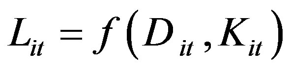
Generally, most of the studies (if not all) on efficiency of Rural and Community Banks have utilised the non parametric Data Envelopment Analysis (DEA) approach (see [16])4. The performance or technical efficiency of RCBs has been defined as the ability of an RCB to transform (multiple) resources into (multiple) financial resources [17]. We follow the banking literature and use the intermediation approach proposed by Sealey and Lindley [18] to define inputs and outputs. This intermediation approach treats deposits as inputs and loans as output. In this study, we include loans and advances as outputs and deposits, and physical capital (fixed assets) as inputs. In other words, loans and advances of RCBi at time t is given by:
 (1)
(1)
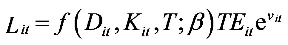
where Lit is loans and advances of RCBi at time t, f(.) is suitable functional form, Dit and Kit are defined as deposits and physical capital for RCBi at time t respectively. We assume that some RCBs may lack the ability to employ existing inputs and technologies as efficiently as possible and consequently produce less than the optimal output. Therefore the actual observable output produced by each RCBi at time t(Lit) is then better described by the following stochastic frontier production function:
 (2)
(2)
T is a time trend common to all RCBs and β is an unknown parameter to be estimated. TEit represent technical efficiency and is defined as the exponential of −uit, where uit > 0 and is a measure of the shortfall of output from the frontier (technical inefficiency) for each RCB in the sample. vit embodies measurement errors, any statistical noise and random variations of the frontier across RCBs.
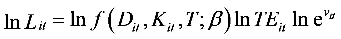
Writing Equation (2) in logarithms form, we have:
 (3)
(3)
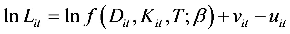
Replacing TEit with exp (−uit), Equation (3) can be reformulated as
 (4)
(4)
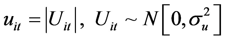
uit > 0, but vit may take any value and is assumed to be a half-normal distribution.
An important issue with regard to the estimation of Equation (4) is the functional form of the production frontier. We apply the Cobb-Douglas specification to characterise the production frontier as:
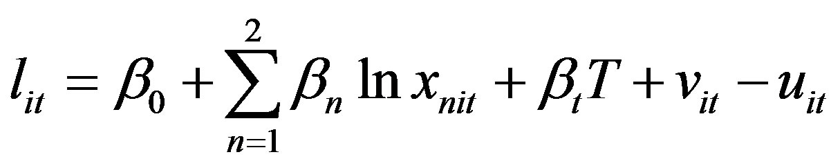 (5)
(5)
where lit represents the logarithm of Lit and xnit denotes an n-th input variable. For convenience, the Cobb-Douglas production frontier function in Equation (5) can be rewritten as:
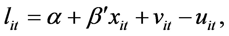 (6)
(6)
where the proxy for technical change T is included in .
.
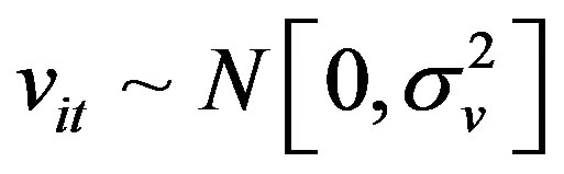
Equation (6) is a baseline pooled frontier model [19]. Given the following distributional assumptions: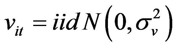 ;
;  and, vit and uit are distributed independently of each other and of the regressors, Equation (6) can be estimated by maximum likelihood (ML) method. Equation (6) does not assume any RCB-specific effects and also does not have the ability to distinguish between inefficiency and unobserved heterogeneity in the efficiency model or in the production model.
2.1. “True” Random Effects Model
The “true” random-effects model modifies the parameterised model in Equation (6) as follows:
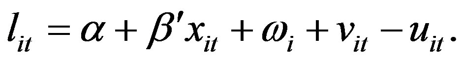 (7)
(7)


 , vit and uit are assumed to be uncorrelated with each other. In the “true” random-effects model,
  (which is assumed to have an iid normal distribution) is a timeinvariant and RCB-specific random term meant to capture unobserved heterogeneity or RCB specific heterogeneity. As proposed by Greene [9,10], we estimate the “true” random effects model by Maximum Simulated Likelihood (MSL) by integrating out
  using Monte Carlo method (see Greene [9,10] for a detailed discussion on the estimation of the model).
2.2. Random Parameter Model
This alternative formulation of the stochastic frontier model allows the function to vary more generally across RCBs. A general form of the random parameters stochastic frontier formulation that models cross RCB heterogeneity in the form of continuous parameter variation may be written as
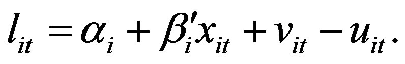 (8)
(8)
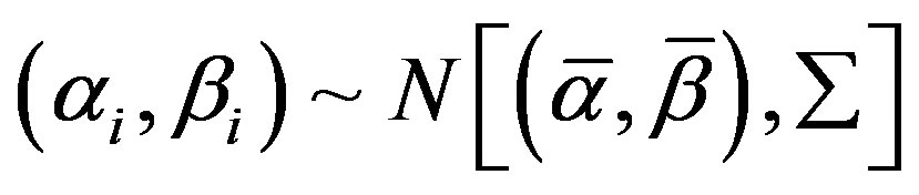
The subvector of the full parameter vector, (αi, βi) is allowed to vary randomly with mean vector  , where
  and
and  (which are assumed to be constant in this specification) are a conformable matrix of parameters to be estimated, and a set of related variables which enters the distribution of the random parameters respectively. Random variation is parameterised in the random vector
  which is assumed to have mean vector zero and known diagonal covariance matrix
  An unrestricted covariance matrix is produced by allowing
  to be a free, lower triangular matrix. In this study, the Cholesky factorisation is used in formulating and manipulating the likelihood function. The random vectors wji will be assumed to be normally distributed, in which case,
 . The underlying covariance matrix for the parameter vector conditioned on the data would then be
  . Since the elements of
  are unrestricted, the variance is assumed to be the known
  which is only a normalization, not a restriction.
This random parameter formulation models cross RCB heterogeneity in the form of continuous parameter variation. In Equation (8), only the (technology) parameters are allowed to vary randomly (normally) across RCBs5. The marginal distributions of the random components, uit and vit are assumed to be common. The model is estimated by maximum simulated likelihood (see Greene [9,10] for a detailed description of structure and computation of the inefficiency estimators).
3. Description and Source of Data
The “true” random effects and random parameter stochastic frontier models discussed in the previous section are applied to an unbalanced panel of 133 RCBs in Ghana for the period 2006-2011. Three sets of variables are required to estimate the models introduced in Section 2. The output variable is (volumes) loans and advancement, and the inputs are deposits, and physical capital (fixed assets). Loans and advancements of the RCBs are measured by the total of microfinance loans; susu loans; salary loans, personal loans, overdrafts and commercial loans. Deposits include the sum of savings and current accounts; susu deposits; fixed deposits and, special deposits. Physical capital of RCB is measured as the value of fixed assets. All input and output variables are measured in millions of Ghana cedis. The trend variable, t = 1, 2, 3, 4, 5, 6 for years 2006, 2007, 2008, 2009, 2010 and 2011. The descriptive statistics of these variables are reported in Table 1. The RCB network in Ghana reaches about 2.8 million depositors and 680,000 borrowers. The RCBs have a market share of 67 percent of depositors and 48 percent of borrowers in rural areas. The dataset is sourced from the Banking Supervision Department of the Bank of Ghana, and the ARB Apex Bank.
4. Empirical Results
Table 2 presents estimated production frontier functions based on the “true” random effects and random parameter models in addition to a baseline model. We estimate the baseline model in order to find out whether the treatment of unobserved heterogeneity is essential for the application to the RCBs dataset in Ghana. Estimated technical inefficiencies and efficiencies are computed using the methods discussed above. To simplify our analysis and comparisons between the different stochastic frontier estimators, we use the direct estimate of inefficiency 
The estimates of λ, σ, σu and σv are reasonable, as are the remaining parameters and the estimated inefficiencies. The estimate of λ is statistically significant suggesting that there is evidence of technical inefficiency in the dataset. However, the estimates of λ = σu/σv for the baseline pooled model is comparatively larger than the two models. The λ value for the base case model falls from
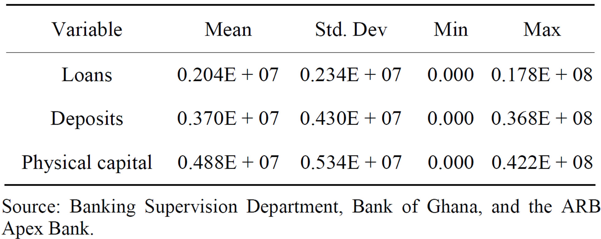
Table 1. Descriptive statistics.
Source: Banking Supervision Department, Bank of Ghana, and the ARB Apex Bank.
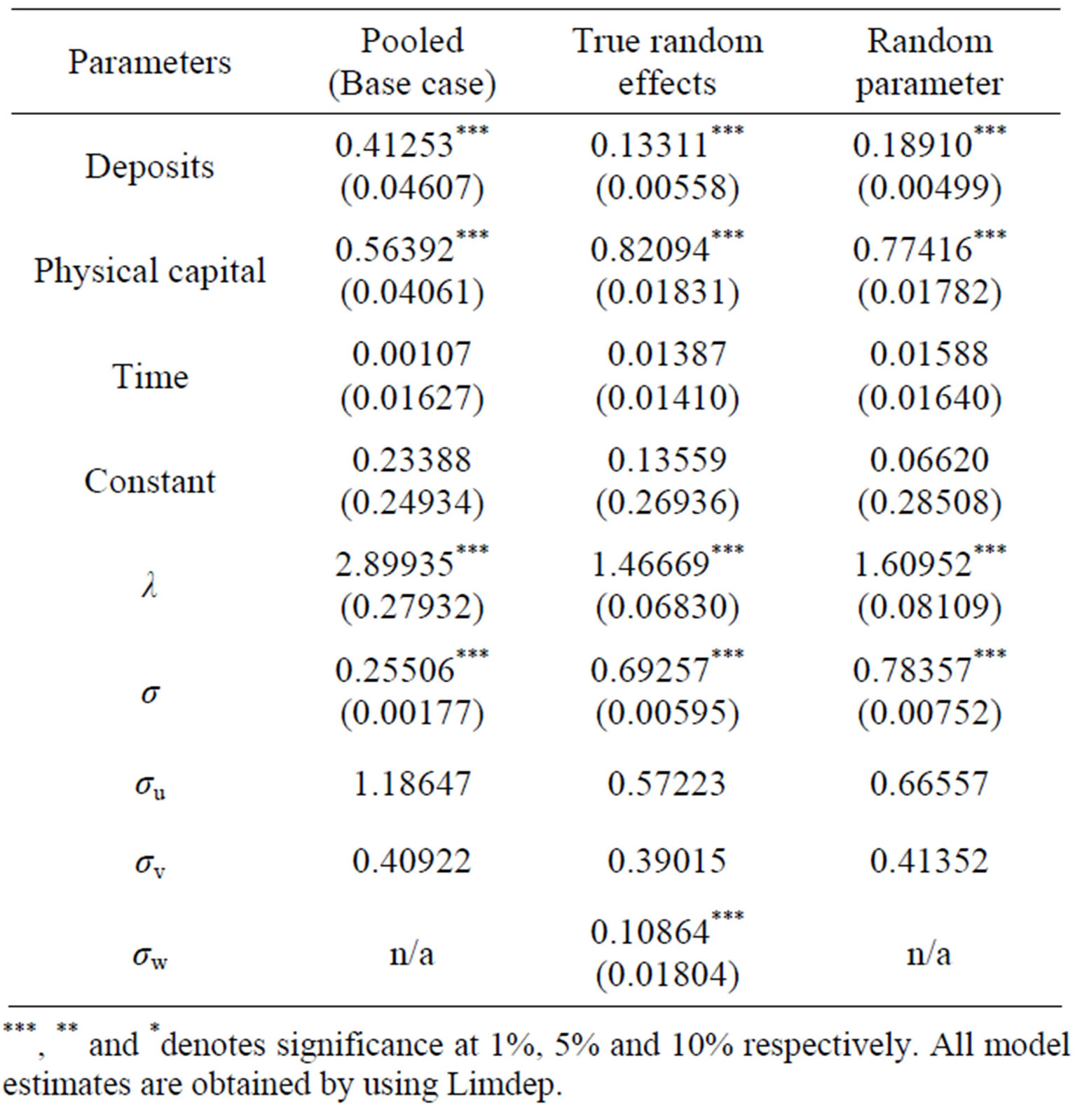
Table 2. Estimated stochastic frontier models (estimated standard errors in parenthesis).
***, ** and *denotes significance at 1%, 5% and 10% respectively. All model estimates are obtained by using Limdep.
2.89 to about 1.46 in the true random effects model. The variance decomposition is dominated by u (σu). The pooled model has the highest σu of 1.18 while σv is fairly even for all models.
The mean inefficiency estimate for the baseline pooled model (that ignores any commonalities or panel data effects) is 0.738781 (74%), while that of the “true” random effects and random parameter models are 0.451396 (45%) and 0.509899 (51%) respectively (see Table 3). Clearly, these inefficiency estimates show that the “true” random effects and random parameter models represent a lower band of inefficiency estimates compared to the baseline pooled model. This is an indication of purging unobserved heterogeneity from the inefficiency estimates in the efficiency model and, production model respectively.
The correlation matrix of the models (see Table 4) confirms the apparent sturdy similarity (shown by the means) between the “true” random effects and random parameter models. For instance, the simple correlation between the “true” random effects and the random parameter models is about 99.9%.
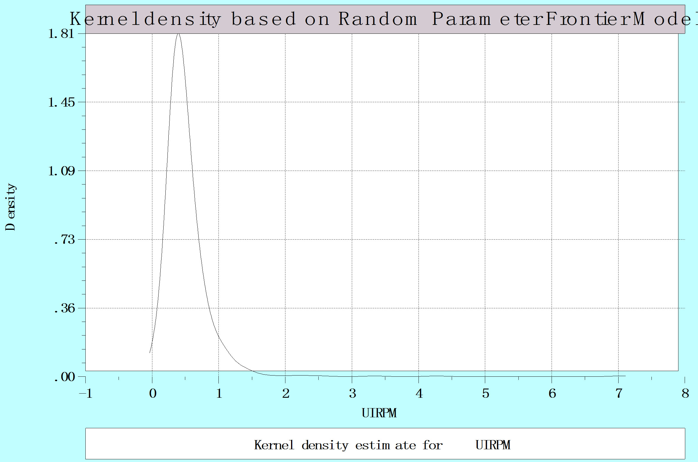
We further analyse the mean and variation of the distributions for estimated inefficiencies of the different models in order to compare their performance. The kernel density estimators show that the mean of the distribution for the “true” random effects and random parameter models is lower compared to the baseline pooled models, while its variance is also considerably lower (see Figure 1). This is a further indication that the “true” random effects and random parameter models appears to consistently treat unobserved heterogeneity in our panel data-
 (a)
(a) (b)
(b) (c)
(c)
Figure 1. Estimated kernel densities for pooled, “true” random effects and random parameter models.
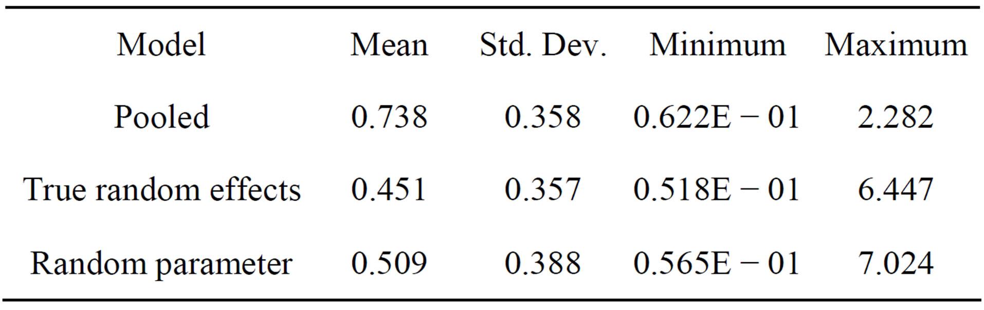
Table 3. Descriptive statistics for estimated inefficiencies.
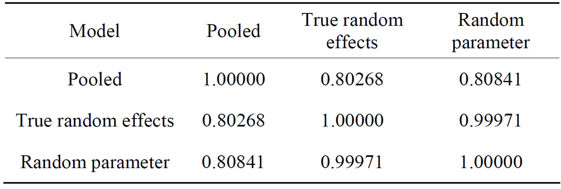
Table 4. Correlation matrix for estimated inefficiencies.
set, be it in the inefficiency model or the production model in our panel data set.
Table 5 shows the average technical efficiency estimates for RCBs in Ghana over the 2006-2011 period. Average technical efficiency of the RCBs in Ghana as a whole is 66% for the “true” random effects model, and 63% for the random parameter model. There is however no substantial differences in efficiency levels and trend over the 2006-2011 period for the two models. Both stochastic frontier models show a steady increase in efficiency levels from 2006 to 2008, followed by a decrease from 2008 to 2010 and a marginal increase from 2010 to 2011. The period (2006-2008) of increasing efficiency levels is associated with an increasing amount of deposits, loans and advances. The growth rate of borrowers showed a generally increasing trend during the period. This is also the period over which the Rural Financial Services Project was implemented. During the 2006- 2008 period, both deposits and loan balances show a positive growth trend, and loan balances grew at a much faster rate, indicating the success of RCBs in increasing lending during this period of increasing efficiency.
5. Conclusions
This paper estimates a “true” random effects stochastic model that controls for unobserved heterogeneity in the inefficiency model, and a random parameter model that accounts for unobserved differences in technologies (parameter heterogeneity) that might be inappropriately labeled as inefficiency respectively. An application of these models is presented using an unbalanced panels of 133 RCBs in Ghana from 2006-2011. The levels of technology for RCBs are different but the technology is well known and is being continuously dispersed under a computerisation project. We compare the results of these two models with regard to the inefficiency estimates and dispersion, and we also measure pure technical efficiency
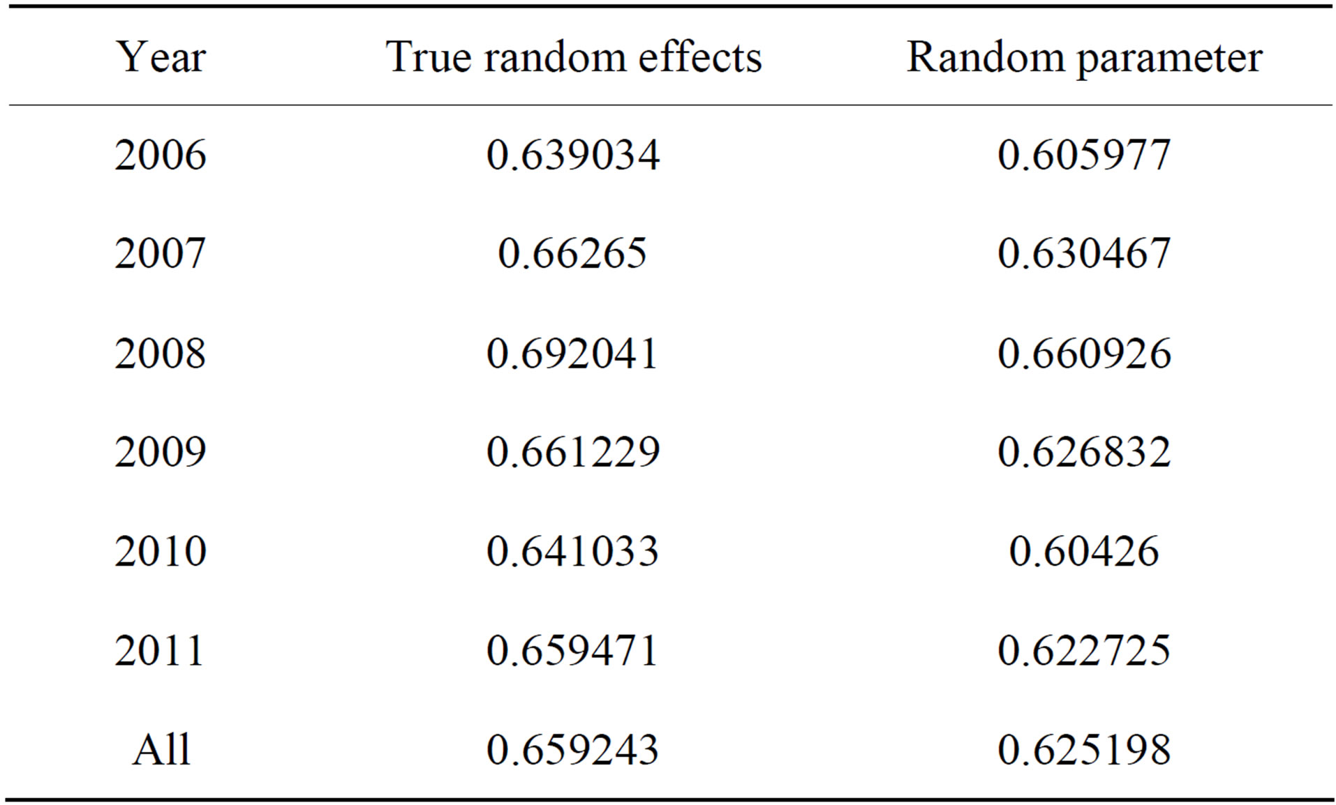
Table 5. Average technical efficiency estimates, 2006-2011.
or performance of the RCBs over the period.
Using loans and advances as output, and volume of deposits, physical capital as inputs, our results show that the true random effects and random parameter models address the issue of unobserved heterogeneity, in the inefficiency term or in the production technology when compared to a baseline pooled model. This is confirmed by the kernel density estimators for inefficiency estimates. Our results also show that average technical efficiency of RCBs in Ghana as a whole is 66% for the true random effects model, and 63% for the random parameter model. Both models indicate increases in efficiency levels from the 2006-2008 period, followed by a decrease in the 2008-2010 period, and a marginal increase from 2010 to 2011. The epoch of increasing efficiency levels is associated with a positive growth trend for deposits and loan balances, but loan balances grow at a much faster rate, indicating a success of RCBs in increasing lending during this period.
REFERENCES
- V. Sena, “The Frontier Approach to the Measurement of Productivity and Technical Efficiency,” Economic IssuesStoke on Trent, Vol. 8, 2003, pp. 71-98.
- L. R. Murillo-Zamorano, “Economic Efficiency and Frontier Techniques,” Journal of Economic Surveys, Vol. 18, No. 1, 2004, pp. 33-77. http://dx.doi.org/10.1111/j.1467-6419.2004.00215.x
- H. O. Fried, C. A. K. Lovell and S. S. Schmidt, “The Measurement of Productive Efficiency and Productivity Growth,” Oxford University Press, Oxford, 2008. http://dx.doi.org/10.1093/acprof:oso/9780195183528.001.0001
- W. H. Greene, “LIMDEP Version 9.0: Econometric Modeling Guide 1 and 2,” 2007.
- R. Kneller and P. A. Stevens, “Frontier Technology and Absorptive Capacity: Evidence from OECD Manufacturing Industries,” Oxford Bulletin of Economics and Statistics, Vol. 68, No. 1, 2006, pp. 1-21. http://dx.doi.org/10.1111/j.1468-0084.2006.00150.x
- M. Henry, R. Kneller and C. Milner, “Trade, Technology Transfer and National Efficiency in Developing Countries,” European Economic Review, Vol. 53, No. 2, 2009, pp. 237-254. http://dx.doi.org/10.1016/j.euroecorev.2008.05.001
- K. G. Iyer, A. N. Rambaldi and K. K. Tang, “Efficiency Externalities of Trade and Alternative Forms of Foreign Investment in OECD Countries” Journal of Applied Econometrics, Vol. 23, No. 6, 2008, pp. 749-766. http://dx.doi.org/10.1002/jae.1024
- C. Mastromarco and S. Ghosh, “Foreign Capital, Human Capital, and Efficiency: A Stochastic Frontier Analysis for Developing Countries,” World Development, Vol. 37, No. 2, 2009, pp. 489-502. http://dx.doi.org/10.1016/j.worlddev.2008.05.009
- W. Greene, “Distinguishing between Heterogeneity and Inefficiency: Stochastic Frontier Analysis of the World Health Organization’s Panel Data on National Health Care Systems,” Health Economics, Vol. 13, No. 10, 2004, pp. 959-980. http://dx.doi.org/10.1002/hec.938
- W. Greene, “Reconsidering Heterogeneity in Panel Data Estimators of the Stochastic Frontier Model,” Journal of Econometrics, Vol. 126, No. 2, 2005, pp. 269-303. http://dx.doi.org/10.1016/j.jeconom.2004.05.003
- M. Filippini, N. Hrovatin and J. Zorić, “Cost Efficiency of Slovenian Water Distribution Utilities: An Application of Stochastic Frontier Methods,” Journal of Productivity Analysis, Vol. 29, No. 2, 2008, pp. 169-182. http://dx.doi.org/10.1007/s11123-007-0069-z
- J. Carroll, C. Newman and F. Thorne, “A Comparison of Stochastic Frontier Approaches for Estimating Technical Inefficiency and Total Factor Productivity,” Applied Economics, Vol. 43, No. 27, 2011, pp. 4007-4019. http://dx.doi.org/10.1080/00036841003761918
- L. Orea and S. C. Kumbhakar, “Efficiency Measurement Using a Latent Class Stochastic Frontier Model,” Empiriccal Economics, Vol. 29, No. 1, 2004, pp. 169-183. http://dx.doi.org/10.1007/s00181-003-0184-2
- C. O’Donnell and W. Griffiths, “Estimating State Contingent Production Frontiers” Working Paper Number 911, University of Melbourne, 2004.
- ARB Apex Bank Limited, “Various Years. Annual Reports,” Accra, 2006-2012.
- D. Khankhoje and M. Sathye, “Efficiency of Rural Banks: The Case of India,” International Business Research, Vol. 1, No. 2, 2008, pp. 140-149.
- A. Bhattacharyya, C. Lovell and P. Sahay, “The Impact of Liberalization on the Productive Efficiency of Indian Commercial Banks,” European Journal of Operational Research, Vol. 98, No. 2, 1997, pp. 332-345. http://dx.doi.org/10.1016/S0377-2217(96)00351-7
- C. W. Jr. Sealey and J. T. Lindley, “Inputs, Outputs, and a Theory of Production and Cost at Depository Financial Institutions,” Journal of Finance, Vol. 32, No. 4, 1977, pp. 1251-1266. http://dx.doi.org/10.1111/j.1540-6261.1977.tb03324.x
- D. Aigner, C. Lovell and P. Schmidt, “Formulation and Estimation of Stochastic Frontier Production Function Models,” Journal of Econometrics, Vol. 6, No. 1, 1977, pp. 21-37. http://dx.doi.org/10.1016/0304-4076(77)90052-5
Appendix
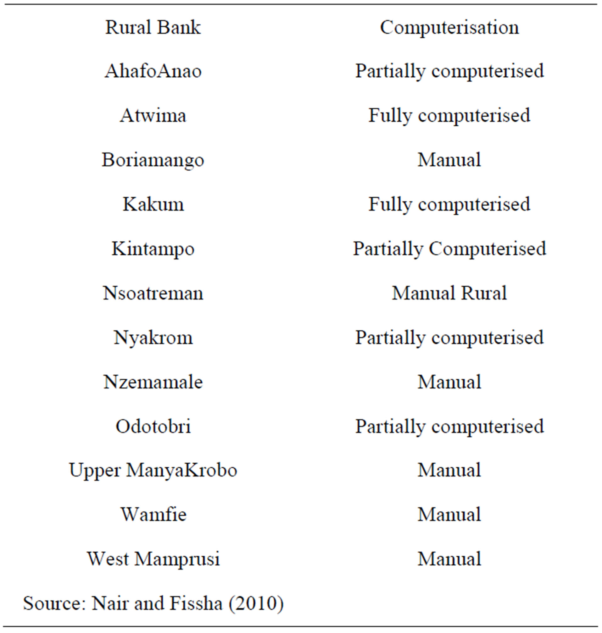
Table A1. Levels of computerisation for a sample of 12 RCBs.
NOTES
1The reasons for these are twofold. First, the stochastic frontier method has deep roots in the economic theory. In this case, efficiency is measured as the distance from a best practice frontier (or the boundary of the production possibility frontier), computed in accordance with the axioms of the production theory. Second, the concept of a distance from the standard allows us to operationalise the concept of inefficiency, providing ready to use information for policy makers.
2The Ghana Rural Banks Computerisation and Interconnectivity Project (GRBCIP) is financed by the Millennium Challenge Corporation (MCC) and will provide support for computerising all RCBs. The program is being built on the RCB computerisation program initiated by the Rural Financial Services Project (RSFP).
3To the best of our knowledge there is no robust empirical study on RCBs in Ghana using stochastic frontier analysis. In the case of RCBs in Ghana, which play a special role in serving the financial needs of the rural dwellers and also an agent of development, improved efficiency of the RCBs would lead to provision of better and relevant services that address the peculiar needs of the rural dweller; greater security; and financial and macroeconomic stability.
4The reasons are not farfetched-given an appropriate dataset, the DEA is fairly easy to estimate. However, the DEA approach does not treat unobserved or parameter heterogeneity.
5The model allows, all at once, half normal or truncated normal distribution for uit and firmwise and/or time wise heteroscedasticity in uit. The model form allows parameters to be random in all three parts of the specification with the single restriction that only the variance of the disturbance, vit is assumed to be constant. This model form does not accommodate heteroscedasticity in vit (see Greene [4]).