Smart Grid and Renewable Energy
Vol.2 No.2(2011), Article ID:4960,10 pages DOI:10.4236/sgre.2011.22015
Medium-Term Electric Load Forecasting Using Multivariable Linear and Non-Linear Regression
![]()
1Department of Electronics and Communications, Ahlliya Amman University, Amman, Jordan; 2Department of Electrical Engineering, The Hashemite University, Zarqa, Jordan.
Email: {nabushik, fkarmi}@ammanu.edu.jo, aloquili@hu.edu.jo
Received November 2nd, 2010; revised March 29th, 2011; accepted April 3rd, 2011.
Keywords: Medium-Term Load Forecasting, Electrical Peak Load, Multivariable Regression, Time Series
ABSTRACT
Medium-term forecasting is an important category of electric load forecasting that covers a time span of up to one year ahead. It suits outage and maintenance planning, as well as load switching operation. We propose a new methodology that uses hourly daily loads to predict the next year hourly loads, and hence predict the peak loads expected to be reached in the next coming year. The technique is based on implementing multivariable regression on previous year’s hourly loads. Three regression models are investigated in this research: the linear, the polynomial, and the exponential power. The proposed models are applied to real loads of the Jordanian power system. Results obtained using the proposed methods showed that their performance is close and they outperform results obtained using the widely used exponential regression technique. Moreover, peak load prediction has about 90% accuracy using the proposed methodology. The methods are generic and simple and can be implemented to hourly loads of any power system. No extra information other than the hourly loads is required.
1. Introduction
The fact that there are many variables contributing to the electric load makes accurate prediction of electric load a difficult process. These variables involve “uncertainty” and have no direct relation with the final load. Moreover, the load is characterized to be nonlinear and non-stationary process that can undergo rapid changes due to weather, seasonal and macroeconomic variations. So linearization of the load contributes to making many of the classical prediction models inappropriate [1,2].
From the forecasting point of view, the utility/company seeks to operate the power system such that a match is achieved between the electric energy demand and supply. This implies that the more accurate the forecast, the more efficient the operation and management of the power system.
Medium term load forecasting covers a time span of (1 - 12 months) [3]. This type of forecasting depends mainly on growth factors, i.e. factors that influence demand such as main events, addition of new loads, seasonal variations, demand patterns of large facilities, and maintenance requirements of large consumers. Moreover, this type of forecast uses hourly loads for prediction of the peak load of days or for the weeks ahead. With this information it can be decided to whether take certain facilities/plants for maintenance or not during a given period of time. This will also help to plan major tests and commissioning events, and determine outage times of plants and major pieces of equipment. The analysis methods used for this type of forecast are similar to the short term forecast. However, it should be remarked that the sensitivity of medium-term forecasting on power system operations is less than that of the short-term forecasting [4].
Since the electric load varies continuously in time, it is considered to be a time series. This enables applying different time series techniques and methodologies to predicting future loads based on the available historical data of the loads.
Time series techniques are based on the assumption that the data have an internal structure, such as autocorrelation, trend, or seasonal variation. Time series forecasting methods detect and explore such a structure [4,5]. The objective of this paper is to develop and implement a new technique that is based on a non-linear model using multivariable regression. This will work as a filtering process to explore the structure of the load behavior, as well as, to enable prediction of future loads. In this paper, the time series approach is adopted, however, we propose establishing a fit to an exponential model that takes into account the previous years’ hourly loads.
Electric companies/utilities use mostly simple forecasting models like linear regression and simple econometric models of one or two parameters. However, the current trend now is to apply multiple regression forecasting models especially to large systems [6,7]. Multiple regression in addition to ARMAX models showed also good performance [8] and they were applied to both electric load and energy forecasting [9,10].
As a matter of fact the majority of forecasting models use statistical techniques or artificial intelligence algorithms such as regression, neural networks, fuzzy logic, and expert systems. The end-use and econometric approach is broadly used for mediumand long-term forecasting. A variety of methods, which implement the similar day approach, various regression models, time series, neural networks, statistical learning algorithms, fuzzy logic, and expert systems, have been developed and are available for short-term forecasting [4,5,9,10].
The forecasting category belonging to quantitative methods are based on mathematical formulation and include: regression analysis, decomposition methods, exponential smoothing, and the Box-Jenkins methodology [11-13]. The research carried out in this paper belongs to this category, i.e. quantitative methods.
This paper is organized as follows: in Section 2, the description of the multivariable regression model is illustrated followed by the introduction of the exponential power model. In Section 3 the developed technique is explained, and in Section 4, results of implementing this technique to the Jordanian power system are discussed and analyzed using several error and accuracy indicators. A comparison of the results obtained using the proposed method with those obtained using the exponential regression method is also demonstrated. Section 5 presents the final outcomes and conclusions of this study.
2. The Models
When time series analysis is in forecasting, past information is used, in conjunction with a forecasting model, to predict future values. This becomes an optimization problem. In general, this process can be expressed as the search for or synthesis of a function f which leads to the prediction accordingly [14]:
 (1)
(1)
where,
 is the estimated loads for the next time spanN is the signal length = 8760 hours
 are the multiple variables (m = 1,2,
  l,
l, )
)
 are the model parameters to be computed (i = 1,2,
 , P)
, P)
λ is the number of years span considered in the forecasting process.
Practically speaking, forecasting becomes a problem of approximating a given function as precisely as possible while being able to quantify the performance of forecasting error [15,16].
In this research we propose using the previous year’s yearly hourly loads in conjunction with multivariable regression to find the forecast of the next year hourly loads. Three models are investigated: a) Modeling the next year’s load as a linear function of multivariable (previous year’s hourly loads), b) as a nonlinear function of previous year’s hourly loads, and c) as a power exponent of previous year’s hourly loads. The mathematical formulation of these models is derived in the subsequent sections.
2.1. Multivariable Regression
Multiple regressions are used in load forecasting when the predictor variable y is set to be a function of more than one variable. A linear regression model is given as:
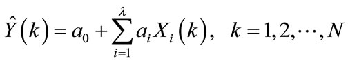 (2)
(2)
where,
 is the estimated loads for the next yearN is the signal length = 8760 hours
 are the multiple variables
 are the model parameters to be computed (i = 0,1,
 , l)
, l)
λ is the number of years span considered in the forecasting process.
The linear model for a time span l = 1, reduces to:
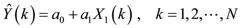 (2a)
(2a)
The non-linear multiple regressions assume that the estimates of loads  have a non-linear relationship with the multiple variables
 . It should be noted that the selection of the multiple variables is open and unlimited to a restricted set. For short-term load forecasting, they can represent the temperature, the wind speed, the cloud density, etc. In this research the selection was directed to the hourly loads of the year. So
  were selected to represent the previous year’s hourly loads.
An mth order multivariable polynomial regression may take the following form:
 (3)
(3)
where,
 are the unknown parameters to be computed with [i = 0,1,
 ,l, and j = 0,1,
 ,m]
,m]
If the estimated hourly load data is assumed to depend on the previous year hourly loads data, then the model of Equation (3) may be written as:
 (3a)
(3a)
The unknown parameters  are found by minimizing the Mean Squared Errors (MSE) between original and estimated values is given as:
 (4)
(4)
The unknown parameters are found using the following equation:
 (4a)
(4a)
2.2. The Exponential Power
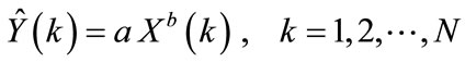
This model gives an estimate of the current value of a given signal through modeling it as an exponential function of previous year’s hourly loads. If we select the previous year dependency, then the model is mathematically described as:
 (5)
(5)
where,
 is the estimated loads for the next yearN is the yearly hours = 8760 hours
 is the previous year’s loads at the kth hour.
a ,b are the model parameters to be computed It is essential to replace the data by their natural logarithm (ln = loge), this will transform Equation (5) to a linear form, given by:
 (5a)
(5a)
It can be seen that  implying that
 . The objective is to find optimum values for a, and b. Hence, by minimizing the (MSE) between original and estimated values is given as:
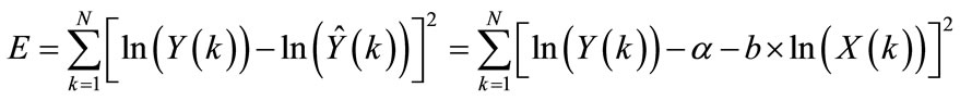
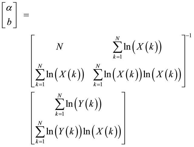
This objective is attained by setting the partial differentials of E with respect to a, and b equal to zero. This will lead to the following:
The unknown coefficients can be found using:
 (7)
(7)
Hence, the optimum values are:
 (7a)
(7a)
Therefore the model parameters a, and b, are assessed such that
 (7b)
(7b)
3. The Proposed Technique
3.1. Modeling
The proposed load forecasting technique can be applied to assess the medium term load forecasting in any power system. A simple block diagram that represents the modeling phase of the proposed methodology is illustrated in Figure 1.
This figure shows that the input variables are given by previous year’s hourly loads , (m = 1,2,
 l, and k = 1,2,
 ,8760). The computed model parameters, are used in conjunction with the actual load
  to provide the hourly load forecast
 . The forecasted loads are then subtracted from the actual recorded hourly loads. This will result in the noise added or the random part of these loads. This analysis is performed for previously known loads, and results are used to define the pattern and behavior of the R component, in addition to the characterization of the computed parameters of different models used.
In fact we can use Signal to Noise ratio as a measuring metric. It is shown in a following part of this paper that the SNR for the proposed models is about 21 dB. The next step is, obviously, to use obtained results to estimate
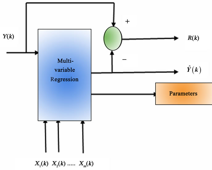
Figure 1. Multi-variable regression modeling.
or forecast the next time span unknown loads.
3.2. Parameters Estimation
The estimation stage is based on three factors:
1) The signal to noise ratio (SNR) between the recorded hourly loads and their corresponding random loads R. This is given as:
 (8)
(8)
2) The model parameters computed in the previous phase, to compute .
.
3) The energy growth model which is a polynomial model used to fit the recorded yearly energies. Here, we can also use the sum of hourly loads to represent acceptable energy consumption for certain power systems.
The above factors can then be employed to compute the medium term forecast, for k = 1,2, ,8760, according to the following steps:
1) Knowing the average SNR, and the energy forecast of the recorded load, then the energy of the R(k) component for the next time span is computed.
2) Use the estimated parameters to compute the model-based estimation of loads .
.
3) The hourly load forecast is found by adding results of 1, and 2 above, resulting in an estimation given by 
3.3. Load Forecasting
In this research, the forecasting process using multivariable method is restricted to the time span of one year. The adopted load forecasting procedure based on this time span, i.e. , involves the following steps, which are illustrated in Figure 2:
a) Process the hourly loads of previous year using the specific regression model to compute model parameters,

Figure 2. Forecasting process for time span l = 1.
estimated load.
b) Compute the energies , and
, and .
.
c) Compute the random component , and the energy of this component
 .
.
d) Compute signal energy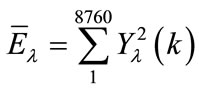 , and extrapolate to find the value at the next time span
 .
.
e) Find an estimate of the noise energy for the next span based on Equation (8), such that 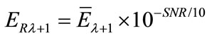
f) Find the estimate of R for the next time span using .
.
g) Find the initial estimate of the load in the next span as: 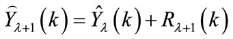
h) Find the required an estimate of the load 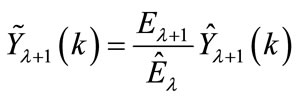
3.4. Error Performance
Many error measures exits which are defined based on recorded (actual),  , and estimated loads,
  , k=1,2,
  ,8760. The following were used in this research:
a) The absolute normalized error ( ), which is computed based on the following equation:
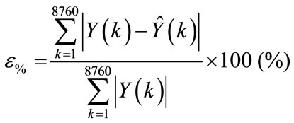 (9a)
(9a)
The absolute percentage error (APE) ( ), which is computed based on the following equation:
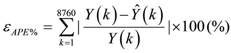 (9b)
(9b)
b) The average of the absolute error ( av), which is computed based on the following equation:
 (9c)
(9c)
4. Implementation to Jordanian System
The hourly loads for the years 1994-2008 were used to explore the characteristics of the Jordanian power system. The three proposed models were applied to the abovementioned loads as explained in the following sections. The first step was to estimate the energy growth of this system.
4.1. Estimation of Energy
The Jordanian system energy growth over the years and the corresponding 2nd and 5th order polynomial fit are shown in Figure 3.
The corresponding equations of the estimated energy ( ) in (MWH) for these fits, with k = 1,2,
 ,8760,
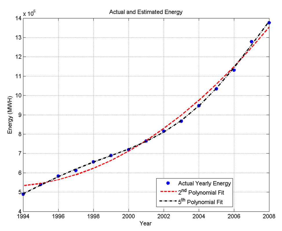
Figure 3. Energy growth and their polynomial fit for the years 1994-2008.
are:
• Second order polynomial:
 (10a)
(10a)
• While, the fifth order polynomial is:
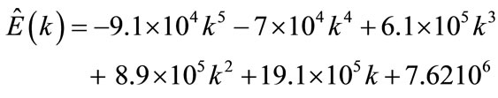 (10b)
(10b)
It is apparent from Figure 3 that a fifth order polynomial will result in a very close prediction values of energy over the years of study. However, the second order fit shows acceptable results and can be used if simpler computations are needed. The polynomial fit will be used to find out unknown future energy values, which are used to compute the associated random or noise component for the particular year as explained in the following sections.
4.2. Linear Model Parameters
Here, the model shown in Equation (2) was used where future load is assumed to depend on the loads of several historical years. The SNR was computed for different values of l between 1-7 years. Results are summarized in Table 1:
Table 1 shows that the time span has little effect on the SNR. In fact the overall average of the SNR is 20.2 dB. The coefficients associated with the time span l = 1 (Equation (2a)) were computed and results are shown in Table 2.
The over all averages for all years are: SNR = 20.9, a0 = 163.6 and a1 = 0.9 It is concluded that the average linear model for l = 1 can be described by the following formula (for k = 1,2 , 8760):
 (11)
(11)
A typical actual hourly loads , and forecasted hourly loads
 , in addition to the noise hourly values
  for a selected year (2004) is shown in Figure 4.
4.3. Polynomial Model Parameters
Here, the model shown in Equation (3a) was used (i.e. l = 1). This selection of l was used to simplify the model and to assure higher load correlation due as the time span l is reduced. Moreover, this selection will enable comparing results of this model with that of the exponential power model.
The SNR was computed when using the third order polynomial model (i.e. P = 3), and results showed that the overall average of the SNR is 20.9, while the optimum model using third order polynomial multivariable regression is given (Equation (3a)) on average, for k = 1,2,  ,8760, as:
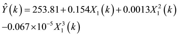 (12)
(12)
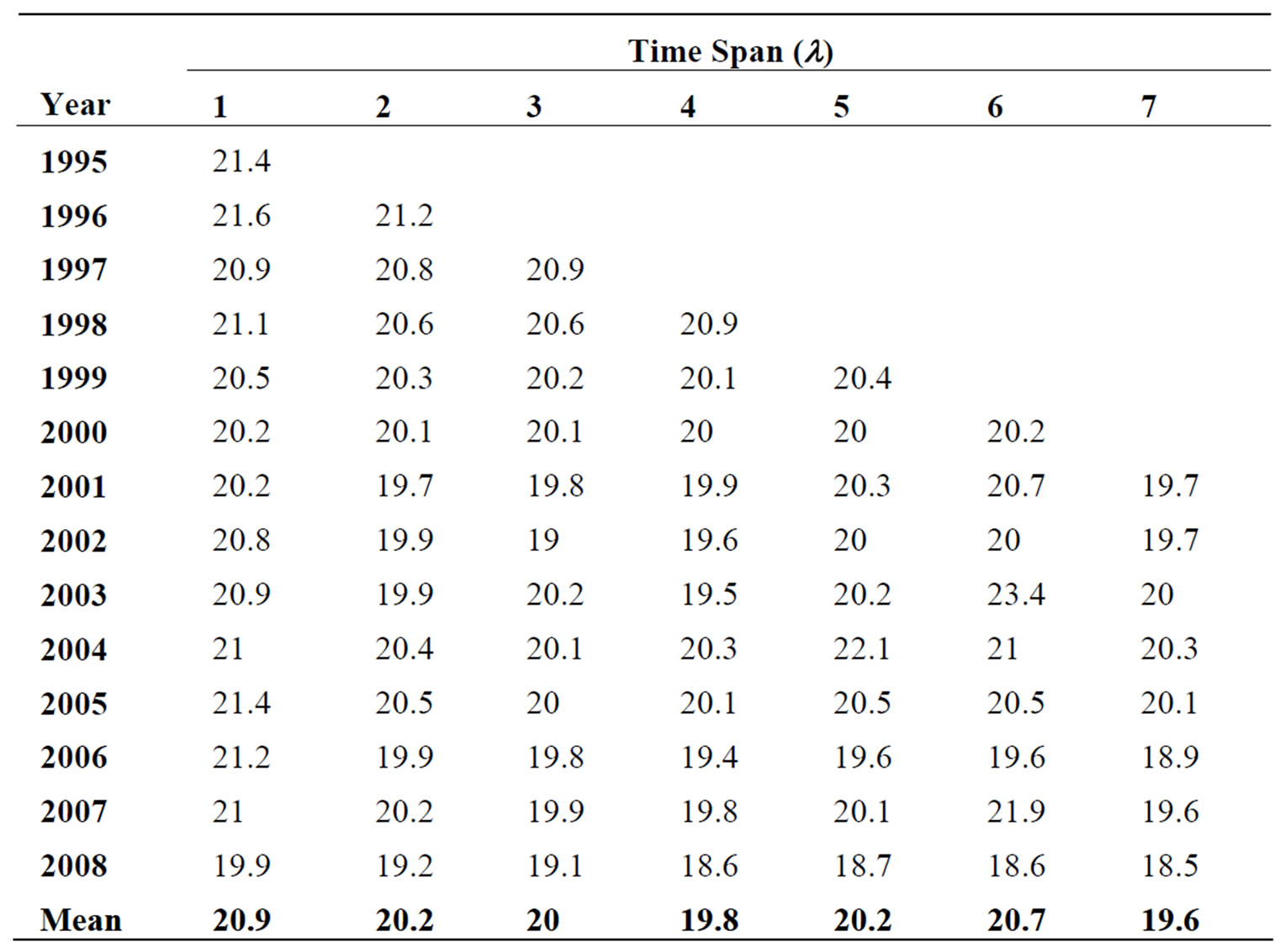
Table 1. Effect of time span (l) on SNR for different years.

Table 2. Linear model coefficients for time span l = 1.

Figure 4. Load components related to linear model analysis for 2004.
4.4. Exponential Power Model Parameters
Here, the model shown in Equation (5) was used with one year span. The SNR values, and the model parameters were computed using the matrix equation given by Equation (7). Results showed that the SNR for the individual years are close, and the average SNR values is about 21 dB. Similarly, the computed model parameters (found by using Equation (7)) have also close values for different years, and it can be concluded that a good model, for k = 1,2, ,8760, would be given by:
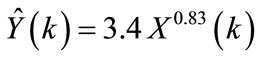 (13)
(13)
It should be emphasized that other time span value can be used, and hence the procedure must be modified accordingly. However, this is out of the scope of this paper and shall be investigated in future research. We shall illustrate using the above procedure to forecast the load of the year 2008 for the three models adopted.
4.5. Forecasting Results
4.5.1. Linear Model
The results of application of the linear model are summarized in Table 3" target="_self"> Table 3. The table shows the errors incurred when applying the linear model and the corresponding yearly peak loads errors. It can be seen that the average error in estimation reaches 9.8% while the absolute error averages to 6.7%. The mean error per hour is about 96 MW. On the other hand the percentage error in peak forecasting is about 5.3% which corresponds to 76.7 MW.
4.5.2. Polynomial Model
The results of application of the third degree polynomial model are summarized in Table 4 which indicates that the errors incurred of the polynomial model are very similar to those obtained for the linear model. It can be seen that the average error in estimation reaches 9.7% while the absolute error averages to 6.4%. The mean error per hour is about 97 MW. On the other hand the percentage error in peak forecasting is about 4.7% which corresponds to 72.2 MW.
4.5.3. Exponential Power Model
The results of application of the exponential power are summarized in Table 5" target="_self"> Table 5. The table shows that the errors incurred of the exponential power vary to a limited extent from those obtained for the linear model. It can be seen that the average error in estimation reaches 10.3% (worse than linear) while the absolute error averages to 4.6% (better than linear). The mean error per hour is about 111 MW. On the other hand the percentage error in peak forecasting is about 9.2% which corresponds to 120 MW (worse than linear).
4.5.4. Comparison with Exponential Regression
A comparison between the proposed methods and the exponential regression method, which is widely used by many electric utilities, was performed. Hourly load data for the period 1994 - 2007 were used to predict the hourly loads of next time span using exponential regression. Results show that the average error incurred is 299 MW corresponding to 20% in the peak load estimation using the exponential regression. For the year 2008, in particu

Table 3. Linear model: overall incurred errors and peak load errors.
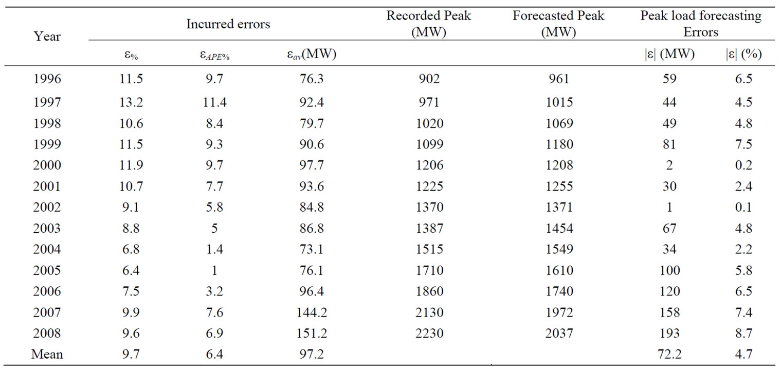
Table 4. Polynomial model: overall incurred errors and peak load errors.

Table 5. Exponential power model: overall incurred errors and peak load errors.
lar, the forecasted peak load was 1 632 MW compared to the actual peak load of 2 230 MW. This corresponds to an absolute error of about 27%. On the other hand, the estimated peak loads using the proposed techniques results in errors in the range of 4.7% - 9.2% (see Tables 3-5). This means that the proposed methods outperform, to a large extent, the exponential regression. It is worth nothing that the large error observed in the forecast of the regression method can be attributed to the fact that this technique performs better when applied to monthly or yearly peak loads rather than hourly loads.
5. Conclusions and Recommendations
We have proposed three models to perform load forecasting based on multi-variable regression (linear, polynomial, and exponential power). These models are generic and can be used in medium-term load forecasting for any power system. Results showed that the performance of the linear and polynomial models perform was close, when applied to the hourly loads of the Jordanian power system for different years. The exponential power model performs close to the linear model, however, due to its more complex nature; it is only applied to a time span of one year. The incurred forecasting errors for the investigated three models is about 10% while the absolute error (APE) ranges between 4.6% (exponential)-to 6.7% (polynomial).
Peak load forecasting results showed that the exponential model performance is far behind the performance of the linear and polynomial models. In fact, the average error in peak load forecasting using the exponential model reaches 9.2% which is almost double the error of the other models. The average incurred error in peak load forecasting using linear model was 5.3%, which is a reasonable percentage. Results also showed that all three methods perform much better than the exponential regression method when hourly loads are used to forecast peak loads.
It was also concluded that the linear model is good and simple and suits the needs of the National Electric Power Company (NEPCO) of Jordan. The application of the linear model can also be extended for different time spans, λ, which will provide deeper insight of the load growth pattern of the Jordanian power system. It should be emphasizes that the information needed by the proposed methodologies is only the hourly loads of the year. This means that weather, demographic, socio/economic and other exogenous data will not be required in the load forecasting process. This is an advantage since various pieces of information within the power utility may not be available, or may have high degree of inaccuracy.
Finally, the authors recommend that when the proposed models are adopted, they need to be tested on a collectively different time spans of hourly loads.
REFERENCES
- D. Bassi and O. Olivare, “Medium Term Electric Load Forecasting Using TLFN Neural Networks,” International Journal of Computers, Communications & Control, Vol. I, No. 2, 2006, pp. 23-32.
- B. Bowerman, R. O’Connell and A. Koehler, “Forecasting, Time Seriesand Regression: An Applied Approach,” Thomson Brooks/Cole, California, 2005.
- E.A Feinberg, D Genethliou, “Chapter 12 Load forecasting”, Applied Mathematics for Power Systems, pp.269- 282. http://www.ams.sunysb.edu/~feinberg/public/lf.pdf
- D. Montgomery, L. Johnson and J. Gardiner, “Forecasting & Time Series Analysis,” McGraw-Hill, New York, 1990.
- J. Rothe, A. Wadhwani and S. Wadhwani, “Short Term Load Forecasting Using Multi Parameter Regression,” International Journal of Computer Science and Information Security, Vol. 6, No. 2, 2009, pp. 303-306.
- H. Hippert, C. Pedreira and R. Souza, “Neural Networks for Short-Term Load Forecasting: A Review and Evaluation,” IEEE Transactions on Power Systems, Vol. 16, No. 1, February 2001, pp. 44-55. doi:10.1109/59.910780
- H. Willis and J. Green, “Comparison Tests of Fourteen Distribution Load Forecasting Methods,” IEEE Transactions on Power Apparatus and Systems, Vol. PAS-103, No. 6, June 1984, pp. 1190-1197. doi:10.1109/TPAS.1984.318448
- H. Yang, C. Ming and C. Huang, “Identification of ARMAX Model for Short Term Load Forecasting: An Evolutionary Programming Approach,” IEEE Transactions on Power Systems, Vol. 11, No. 1, February 1996, pp. 403-408. doi:10.1109/59.486125
- M. Kandil, S El-Debeiky and N. Hasanien, “Long-Term Load Forecasting for Fast Developing Utility Using a Knowledge-Based Expert System,” IEEE Transactions on Power Systems, Vol. 17, No. 2, May 2002, pp. 491-496.
- J. Rothe, A. Wadhwani and S. Wadhwani, “Short Term Load Forecasting Using Multi Parameter Regression,” International Journal of Computer Science and Information Security, Vol. 6, No. 2, 2009
- G. Janacek and L. Swift, “Time Series: Forecasting, Simulation, Applications,” West Sussex: Ellis Horwood Limited, 1993.
- N. Draper and H. Smith, “Applied Regression Analysis,” 3rd Edition, Wiley, New York, 1998.
- K. Schittkowski, “Numerical Data Fitting in Dynamical Systems - A Practical Introduction with Applications and Software,” Kluwer Academic Publishers, Dordrecht, 2002.
- D. Bassi and O. Olivares, “Medium Term Electric Load Forecasting Using TLFN Neural Networks,” International Journal of Computers, Communications & Control, Vol. 1, No. 2, 2006, pp. 23-32.
- S. Bengio, F. Fesant and D. Collobert, “A Connectionist System for Medium - Term Horizon Time Series Prediction,” International Workshop on Applications of Neural Networks to Telecommunications, Stockholm, Sweden, 1995.
- A. Khotanzad and A. Abaye, “ANNSTLF - A Neural Network Based Electric Load Forecasting System,” IEEE Transactions on Neural Networks, Vol. 8, No. 4, 1997, pp. 835-846. doi:10.1109/72.595881