Journal of Water Resource and Protection
Vol. 2 No. 1 (2010) , Article ID: 1190 , 8 pages DOI:10.4236/iwarp.2010.21008
The Analysis of Spring Precipitation in Semi-Arid Regions: Case Study in Iran
1Department of Water Resource Engineering, Faculty of Agriculture, Zanjan University, Zanjan, Iran
2Department of Compute Engineering, Faculty of Engineering, Zanjan University, Zanjan, Iran
E-mails: hosseinalihasaniha@yahoo.com, meghdadi@znu.ac.ir
Received October 13, 2009; revised November 16, 2009; accepted November 24, 2009
Keywords: Iran, Semi-Arid Regions, Precipitation, Drought, Box-Cox Transformations Method, Arima Model
ABSTRACT
In this study, Zanjan from Iran has been chosen from among all the semi-arid regions of world, which has Synoptic station and statistical data since 1955. Spring and monthly precipitations are also provided in the period of 1956-2005. First, all data has been controlled by double mass method with the help of adjacent stations, and then it was normalized by the box-cox transformations method. The global SPI index was calculated for all months and spring, also drought and wet periods were determined and finally compared. In the drought category view, spring months have represented the great similarities. The moving averages are represented all months and spring’s precipitations such as three years, five years, seven years and nine years are shown. Statistical period was observed and analyzed based on five periods of ten years, and results precipitation with more than 5mm and 10mm has gradually decreased on April. However the number of days with precipitation has increased. The calculated spring precipitations and all of the atmospheric factors represented the dependence of this model to maximum average of spring temperature and relative humidity of spring and winter by the use of multi variable regression method. The predicted precipitation of spring also showed the gradual decline of precipitation in the next 30 years by the arima model.
1. Introduction
The semi-arid regions involve the great part of the earth’s all arid regions. Nowadays, the study of these regions is one on the most important studies; especially in the last two decades, where there is repetitive drought as a result of shortage of precipitations [1]. These shortages have caused some changes that tend to have influence on these regions. The lack of precipitation’s time distribution is one of the features of the regions, so that there is a great degree of precipitations in the seasons other than the required seasons and can not be controlled. The shortage precipitations and repetitive drought in the last two decades made the rural people to immigrate from villages to cities. Also, the cultivating and animal husbandry has been under losses. These immigrations tend to great problems in the cities’ management. The shortage of the precipitations causes some problems in providing beverage water of cities and industries’ water. As a result of this issue stores and dams become dry and the surface of underground canals began to decline in terms of excessive use. Consequently, the study of precipitations trend and acquaintance of their condition in this period is more useful. In this study, our focus is on the spring precipitations in the semi-arid regions of the world.
Semi-arid regions’ importance is because of their capacity of dry farming. Also, the great amount of these regions’ precipitations in the spring become in the form of rainstorm which is out of control. Therefore acquaintance with the precipitations trend of these regions, in terms of number of factors such as amount, rate, continuousness, recurrence, maximum, minimum degree and day of precipitations, can lead to the correct and proper planning [2]. In this respect we can have proper planning of watering and dry farming, filling of dam, saving superficial water sources, distributing of the flood waters, feeding groundwater tables, preventing floods, and overflows, soil protection and watershed.
2. Materials and Methods
2.1. The Study Site
A semi-arid climate or steppe climate generally described
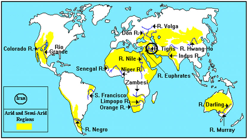
Figure 1. Arid and semi-arid regions of the world.
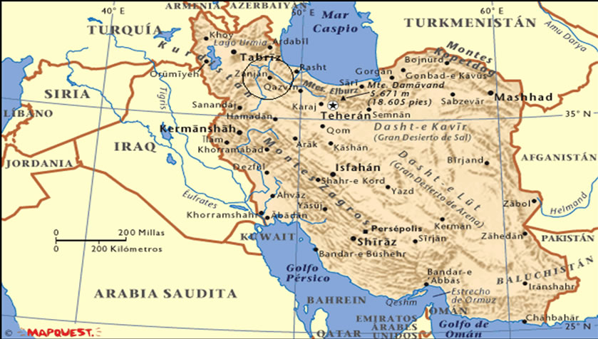
Figure 2. Iran and the location of Zanjan.
climatic regions that received low annual precipitation (250-500 mm or 10-20 in). A more precise definition was given by the Köppen climate classification that treated steppe climates (BS) as intermediates between the desert climates (BW) and humid climates in ecological characteristics and agricultural potential [3]. The Köppen climate classification allows adjustments for temperature and for seasonality of precipitation, effectively excluding forested regions. (In the tables and figures hereafter, the statistics and information belongs to Zanjan).
In this study, we have chosen Zanjan synoptic station where is one of the semi-arid regions of the world in order to observe spring precipitations’ trend in these kinds of areas. Figure 1 represents the semi-arid regions of the world and Figure 2 shows Iran’s geographical map in which Zanjan is specified. Zanjan is located in the North-West of Iran which has 29, 48º longitude and 36, 47º latitude and 1663.6 m height of see surface [4].
The average precipitation in a year reached to 313.1 mm in Zanjan and its average temperature was 10º C in a year, it is necessary to say that the number of glacial days is 117 and the average of evapotranspiration reached to 1025 mm during a year.
Near to 238 million cube meter of the whole amount of Zanjan precipitation that equaled to 1157 million cube meter, was the same as 21 percent of the whole amount of precipitation of this area, in which there was no uses and even in some cases it caused to some material and financial damages such as demolition of agricultural lands and gardens, institutions, buildings, and communication means [1].
2.2. Used Method
2.2.1. Double Mass Method
One of the common graphic methods which are used for making sure of the homogeneity of data is double mass method. This method is usually used for homogenizing of data related to the precipitation and flowing waters [5].
If we had hydrologic time series data in the condition that they had any periodic and non-periodic changes, we could call those data as stationary data. There was always the stationary (fixed) amount of mean and variance if some other identical data was added to them. However, in some cases where the data are not similar we should homogenize them first or make sure they are homogeneous.
2.2.2. The Box-Cox Transformations Method
The most commonly used symmetry-producing transformations are the two closely related functions;
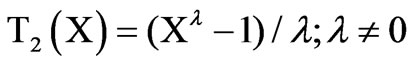 (1)
(1)
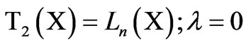 (2)
(2)
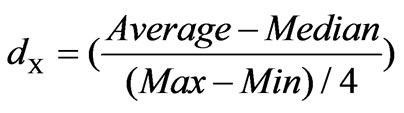
Here “Spread” is some resistant measure of dispersion, such as the “Inter-Quantile range” or “Median absolute deviation”. The Hinkley  is used to decide among power transformations essentially by trial and error, by computing its value for each of a number of different choices for
  [6].
[6].
 (3)
(3)
 (4)
(4)
 (5)
(5)
In the aforementioned method, data are normalized. In other words, data are not normal in %99 of cases and all of the time series of data, and central norms such as mean, median and mode have some differences however they cover one another in the vertex. To analyze data, first we should normalize them.
Normal or Gaussian distribution Law is:
 (6)
(6)
where:
π = 3.14, e = 2.72, µ = mean and σ = variance.
All normal averages are similar and bell shaped and their difference is just in the amount of µ and σ. We assign λ to different numbers in box-cox transformations method formula and then calculate dX. The value of dX is calculated by trial and error. The value of dX is usually acceptable up to 0.01. In order to normalize the data, we do analyzing it near to 0.00 and make sure that all data are normalized %100.
2.2.3. The Standardized Precipitation Index (SPI)
To calculate the SPI, a long-term precipitation record at the desired station was first fitted to the probability of distribution (e.g. gamma distribution), which was transformed into a normal distribution later so that the mean SPI is zero. The SPI might be computed with different time steps (e.g. 1 month, 3 months, and 24 months). Positive SPI values indicated greater than mean precipitation and negative values indicated less than mean precipitation [7] (See table 1).
In this research, we used global SPI Index in order to study the drought, and we calculated the SPI precipitations of the months of spring. The above table represented the SPI Index for categorizing of wet and drought periods.
2.2.4. Stepwise Linear Regression
Linear Regression estimated the coefficients of the linear equation, involving one or more independent variables that best predict the value of the dependent variable. Method selection allowed us to specify how independent variables were entered into the analysis. Using different methods, we could construct a variety of regression models from the same set of variables. In Stepwise Linear Regression, the independent variable not in the equation which had the smallest probability of Analysis of Variance (F), was entered at each step, if that probability was sufficiently small. Variables already in the regression equation were removed if their probability of F became sufficiently large. The method terminated when no more variables were eligible for inclusion or removal [8].
This research used multi variable regression-stepwisemethod that existed in SPSS software in order to reach spring precipitations’ model in terms of all the atmosph eric characteristics.
2.2.5. Arima Forcast Model
Arima fitted a box-jenkins arima model to generate forecosts. Arima stands for autoregressive integrated moving
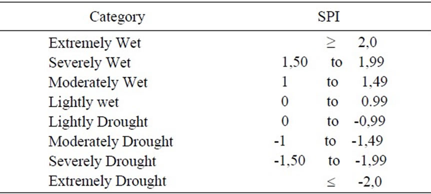
Table 1. The standardized precipitation index values.
average with each term representing steps taken in the model construction until only random noise remained [9].
In this study we used time series and arima model that is a linear model. Ochoa [10] used time series and he divided the method into two groups linear and non-linear models. He mentioned that results of linear models-like arima model – are very better than non-linear models [10].
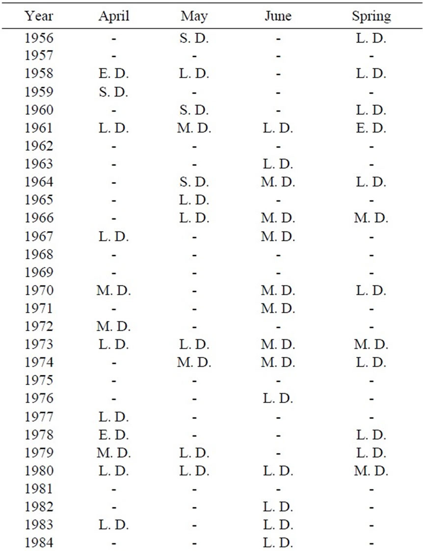
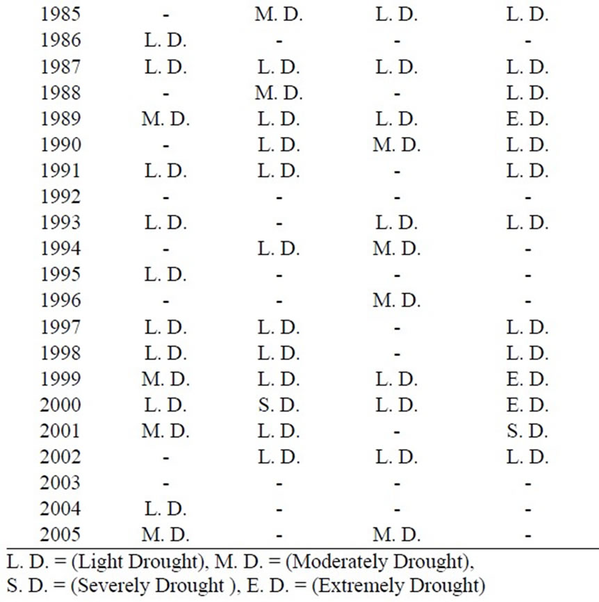
Table 2. Drought category in different periods.

Figure 3. Drought frequency at different periods.
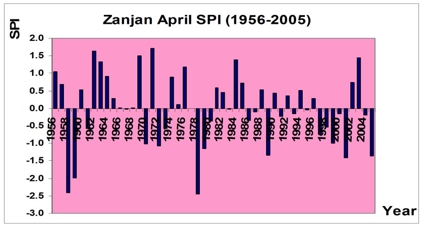
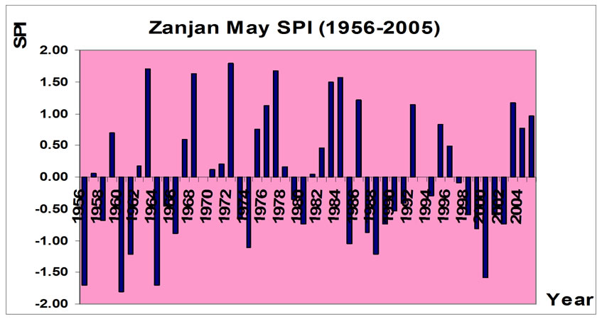

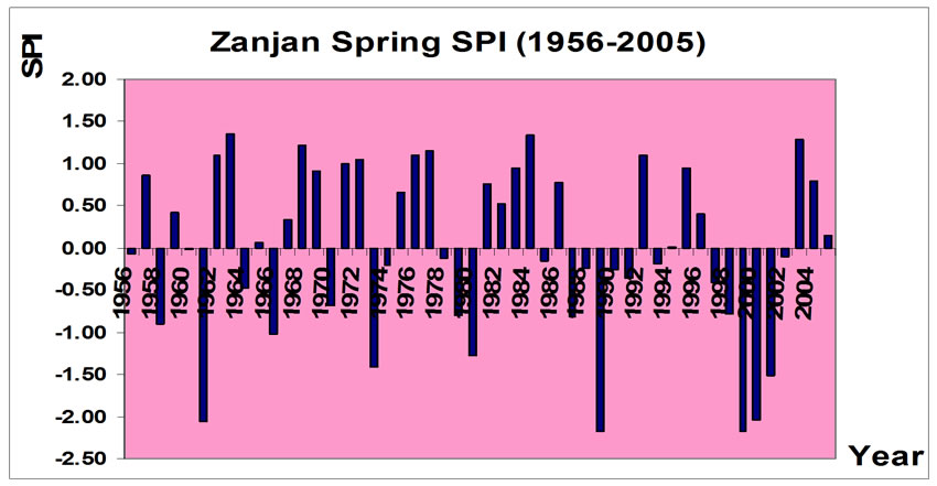
Figure 4. Spring precipitation SPI values in different periods.
This study was done in Zanjan synoptic station using arima model which exists in Minitab software in order to predict the spring 30 years’ precipitations. By using the past fifty year data, we predicted the coming thirty years precipitations of station.
3. Results and Discussion
The opposite situations of drought categories during 1956–2005 are represented. In four periods, light drought category is replicated more than others (Table 2 and Figure 3). On June there were no intensive categories of drought and all ones were in the mean and slight categories. It is necessary to mention that on May there was lack of most intensive categories; however, all of the categories existed on April.
We have drawn the SPI Index’s value on the different time periods in Figure 4. In this figure, the intense of droughts was the most one on April and the last on June. The accumulation of recurrent drought is well cleared in recent years. In [11] the authors used SPI index to investigate meteorological and hydrological drought to see the surface of groundwater tables and to forecast drought. SPI index was not estimated in different time periods. This index has shown a good correlation with GRI index in which it inspects and forecast the conditions of groundwater tables.
The moving averages of precipitations for the periods of 3, 5, 7 and 9 years of April were represented (Figure 5). In the figures you could find the wet and drought periods more clearly and also the gradual decrease of precipitation during fifty years statistical period. As the nine years moving average represented, the amount of accumulated precipitation of April in Zanjan decreased from 60 mm to 40 mm.
The moving average of precipitation of 3, 5, 7 and 9 years during the statistical period has been shown in Figure 6. As the average represents, the amount of accumulative precipitation during spring decreased from 110mm to 80 mm .
The graph of wet and drought periods during 50 statistical years for all months of spring and also for spring itself is shown in Figure 7. Among four trends of drought period’s representations, we confronted with some similarities between May and spring as a whole.
We analyzed the fifty years precipitation of statistical periods (1956–2005) in terms of ten years periods. Figure 8 represented the change of ten years precipitation for different periods. Although all periods showed gradual decrease during the statistical periods, this trend became clearer on April.
Figure 9 represented the accumulative precipitation of different months of spring in terms of percent. As this figure shows, the amount of spring precipitation on April, May and June are respectively %52.90, %37.85 and % 9.25.
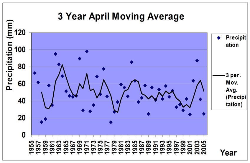
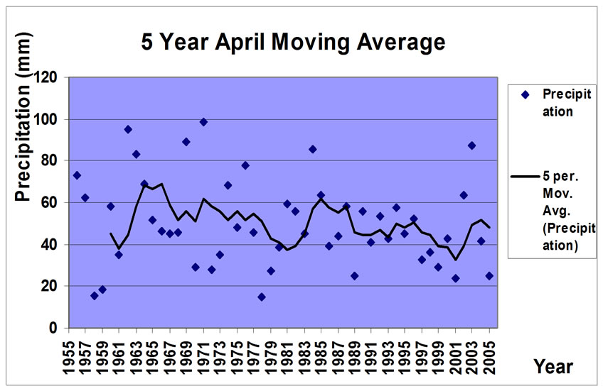
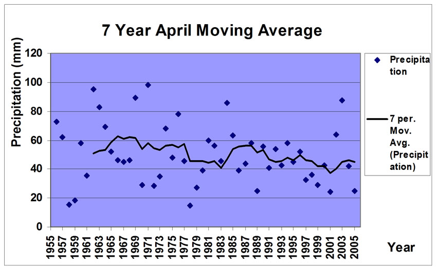
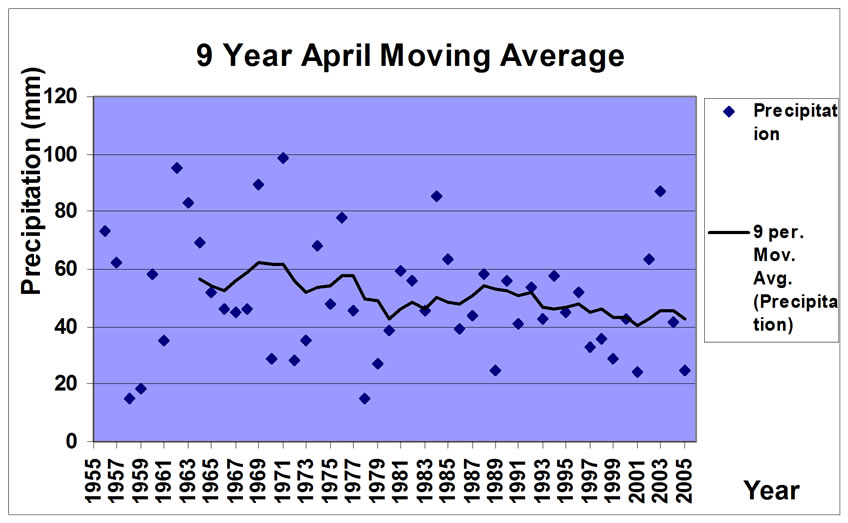
Figure 5. Moving averages of precipitation of April.
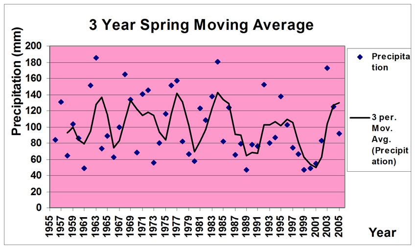
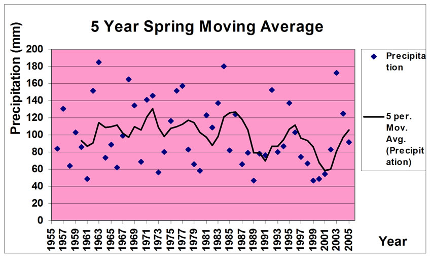

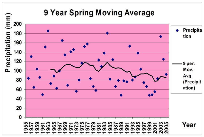
Figure 6. Moving averages of spring.
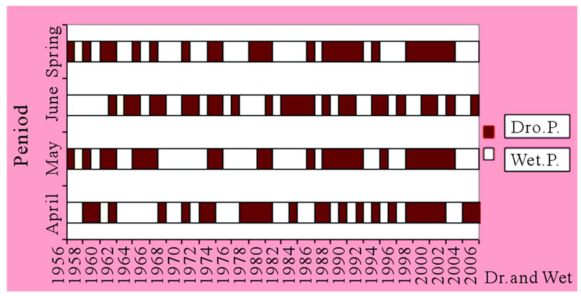
Figure 7. Drought duration in different periods.

Figure 8. Drought process at decimal in different periods.
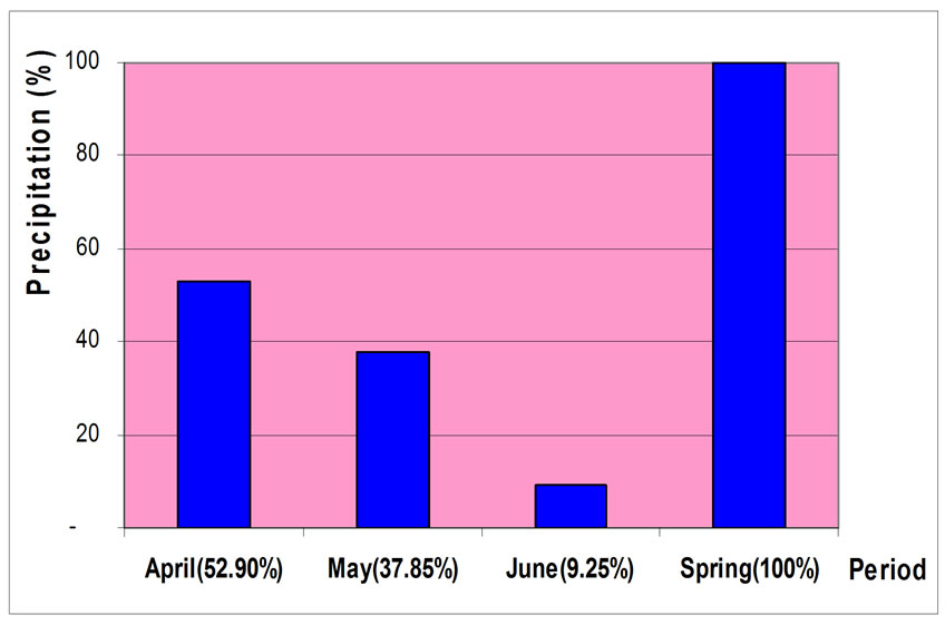
Figure 9. Total precipitation of different hours in April.

Figure 10. The greatest precipitation in 24.

Figure 11. The number of days with precipitation of more than 10mm in April.
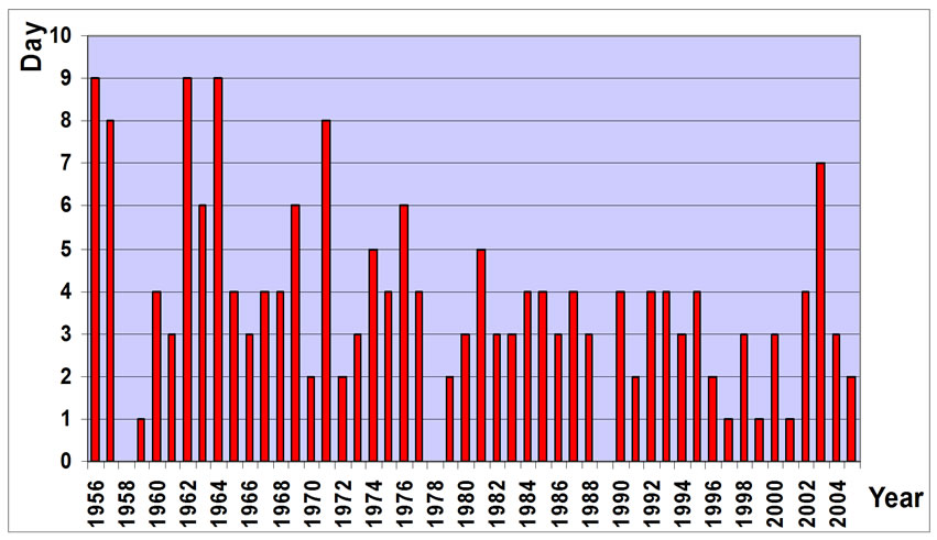
Figure 12. The number of days with precipitation of
more than 5mm in April.
Spring Precipitation = 1.1519 May Precipitation + 53.162Pearson R2 = 0.7113 Periods In Figure 10, you could find maximum precipitation of a day (24 hours) on April during fifty-year statistical period. As figure shows, this precipitation (Maximum precipitation of a day (24 hours) on April has decreased in recent years.
The number of days with precipitation that was more than 10mm in April during the statistical period showed a regular gradual decrease during statistical period. Also you could find the number of days with precipitation of more than 5mm on April and their frequency in Figure 12.
The number of days with precipitation on April during 50 years of statistical period indicated a gradual decline of precipitation during statistical period in Figure 8. however the number of days with precipitation relatively increased.
We calculated the regression of multi variables between accumulative precipitation of spring and all atmospheric factors by Stepwise option of multi variable regression method of SPSS software. The model extracted form this regression marked the dependence of accumulative precipitation of spring to factors such as average of maximum temperature and average of relative humidity.
Spring Precipitation Total = 433.732 – 11.666 spring’s Average of Max. Temperature + 3.590 spring’s Average
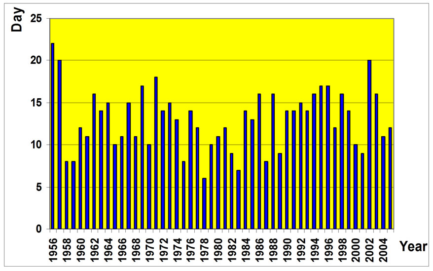
Figure 13. Day with precipitation in April.
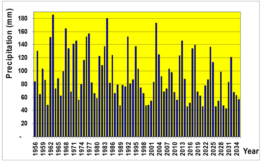
Figure 14. Natural precipitation and our forecast during spring.
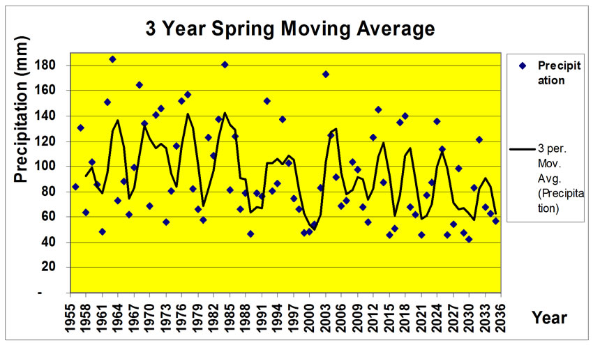
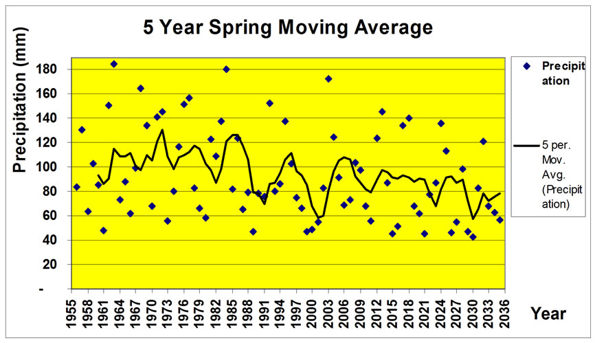
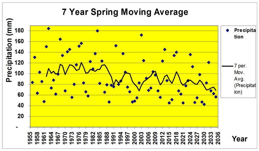
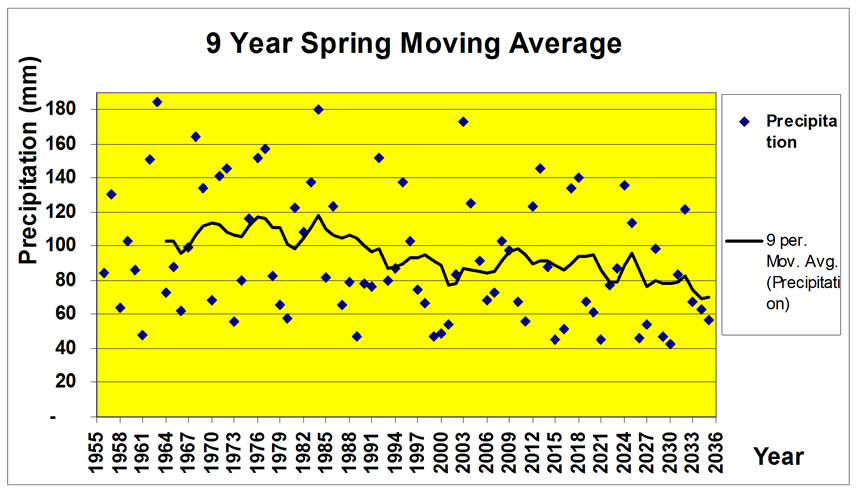
Figure 15. Moving average of natural spring precipitation and our forecast at different periods.
of Relative Humidity (at 09 UTC.) – 2.490 winter’s Average of Relative Humidity (at 03 UTC).
R = 0.772 and R2 = 0.60 We predicted the past accumulative precipitation of Zanjan by the use of 50 years statistics, and also we anticipated 30 years precipitation in this region duringspring by arima model and Minitab software. In Figure 14, you could find the past accumulative precipitations and predicted ones all together and also the graded decline of several accumulative precipitations during last 50 years statistical period and coming 30 years respectively.
The moving average of natural spring predicted in 3, 5, 7, and 9 accumulative precipitations during spring was represented (Figure 15). The wet and drought periods of 80 years and the graded decline of several accumulative precipitations of 110mm to 80mm in 9 years moving average is perceptible through this figure.
4. Conclusions
Authors in [12] have studied region commentary and the management of superficial water sources on semi-arid areas especially it has inspected and forecasted the condition of meteoric – atmospheric - rainfalls. In 2050 (40 years later) meteoric rainfalls decreases up to %20 to %25 in north of Africa, some parts of Egypt, Saudi Arabia, Iran and Syria. Our study has gassed almost the same in 30 future years to decrease %20 in semi-arid areas.
In this paper, we have addressed spring precipitation in semi-arid regions. Spring and monthly precipitations are provided in the late 50 years. Statistical period was observed and analyzed. Results show that the number of days with precipitation has increased. But precipitation with more than 5mm and 10mm has gradually decreased on April. Results represented the dependence of this model to maximum average of spring temperature and relative humidity of spring and winter by the use of Multi Variable Regression method. The predicted precipitation of spring also showed the gradual decline of precipitation in the next 30 years.
REFERENCES
- D. Khalili and A. Ganji, “Analysis of drought with simple time series/disaggregation models, utilizing short record length,” (Persian), Preceding of First National Conference on Drought Mitigation and Water Shortage, Jahad Daneshgahi Kerman and Shahid Bahonar University Publication, Vol. 66, pp. 581–593, 2001.
- WMO (World Meteorological Organization), “World climate news,” The Challenges of Climate Adaptation, Weather Climate and Water (WCN), Vol. 33, pp. 4–11, 2008.
- U. Lohrnann, R. Sausen, L. Bengtssonl, U. Cubasch, J. Perlwitz, and E. Roeckner, “The Koppen climate classification as a diagnostic tool for general circulation models,” Climate Research. Vol. 3, pp. 181–190. 1993.
- WMO (World Meteorological Organization). “Climate: Into the 21st century,” Publisher: Cambridge University press. Editors: William Burrought, Vol. 240, pp. 11–28, 2003.
- A. Alizadeh, Eds., “Principles of applied hydrology,” (in Persian), Astane Ghods, Bonyade Ferhengiy Rezevi Publication, Meshhad, Iran. pp. 451–461, 2006.
- T. Takahiro and H. Yuzo, “A modified box-cox transformation in the multivariate arima model,” In: Journal of the Japan Statistical Society. Vol. 37, No. 1, pp. 1–28, 2007.
- T. B. McKee, N. J. Doesken, and J. Kleist, “The relationship of drought frequency and duration to time scales,” In: Proceeding of the 8th Conference on Applied Climatology, American Meteorological Society, California, 17–22, pp. 179–184, 1993.
- R. W. Simmons and P. Pongsakul, “Preliminary stepwise multiple linear regression method to predict cadmium and zinc uptake in soybean,” In Communications in Soil Science and Plant Analysis, Vol. 35, No. 13, 14, pp. 1815– 1828, 2005.
- P. Brockwell, J. Davis, and A. Richard (Eds), “Introduction to time series and forecasting series,” Spring Texts in Statistics, 2002.
- J. C. Ochoa, “Prospecting droughts with stochastic artificial neural networks,” Elsevier Journal of Hydrology, Vol. 352, pp. 174–180, 2008.
- G. Mendicino, A. Senatore, and P. Versace, “A groundwater resourceindex (GRI) for drought monitoring and forecasting in a mediterranean climate,” In Journal of Hydrology, pp. 5–15, 2008.
- R. Ragab and C. Prudhomme, “Climate change and water resources management in arid and semi-arid regions: Prospective and challenges for the 21st century,” In Bio systems Engineering-Soil and Water, Vol. 81, No. 1, pp. 3–34, 2001.