Atmospheric and Climate Sciences
Vol.3 No.2(2013), Article ID:30790,14 pages DOI:10.4236/acs.2013.32025
Comparison of Gridded Precipitation Time Series Data in APHRODITE and Asfazari Databases within Iran’s Territory
1Department of Physical Geography, Faculty of Geographical Sciences and Planning, University of Isfahan, Isfahan, Iran
2Department of Physical Geography, University of Isfahan, Isfahan, Iran
3Department of Physical Geography, University of Zanjan, Zanjan, Iran
Email: esmailnasrabaadi@gmail.com
Copyright © 2013 Esmail Nasrabadi et al. This is an open access article distributed under the Creative Commons Attribution License, which permits unrestricted use, distribution, and reproduction in any medium, provided the original work is properly cited.
Received December 27, 2012; revised January 30, 2013; accepted February 7, 2013
Keywords: Precipitation Database; Cross-Correlation; Wilcoxon Test; APHRODITE; Asfazari
ABSTRACT
The V1003R1 version of the monthly, seasonal and annual precipitation time series of the Middle East APHRODITE database and Asfazari database within Iranian territory in the time interval 1961 and 2004 were compared with each other. The monthly, seasonal and annual time series of the both databases in most cases show a random behavior and the time series follow a similar pattern with a significant autocorrelation of both databases. Studying cross-correlation between the time series of the two bases indicate that the zero lag significance in the monthly, seasonal and annual time series statistically confirm the coincidence of the peak and fall in the time series of both bases. Wilcoxon Test with 95% confidence confirms significance of the mean difference of the two series. However, there is not enough evidence to confirm the null hypothesis suggesting lack of difference between means of the two series. The statistical-objective analysis of the two bases’ time series indicates that although the series follow a similar course, the estimated precipitation quantity in monthly, seasonal and annual time series of APHRODITE base, except in several monthly time series and in trivial quantities, has been less than the estimated precipitation of Asfazari bases, but the amount of the difference was not constant and did not follow a regular pattern, although this difference has been narrowed in recent years.
1. Introduction
Precipitation data at international, regional and national scale are prepared by different research and commercial institutes and scientists. The main criteria for study of precipitation’s diverse features include trend, frequency change, increase or decrease of rainy days and they give us insight by enriching our knowledge on behavior of climatic processes in the past and present. Therefore, analysis, comparison, evaluation, specification of their weak points and eventual errors are indispensable. Given the availability of diverse evaluation methods and technical qualitative control applied to the data in the centers, comparison of the data quality from different bases in temporal and spatial dimensions will significantly help enrich the knowledge on the data’s common aspects, differences and validity.
The signal output of many physical and financial systems is often characterized by variables which can be both autocorrelated and cross-correlated [1]. The analysis in the temporal domain using such methods as autocorrelation and cross-correlation in time series of different variables as well as in diverse areas is one of the useful and conventional tools in this regard. For example, precipitation’s spatial behavior in the Baden-Wuerttemberg region of Germany from 1997 through to 2004 using Doppler Radar Combined Images data in networks of 4 × 4 km2 and the data of 101 rain gauging stations using cross-correlation were compared. This approach shows that cross correlation varies depending on the chosen quantile. In the lower quantiles, the correlation is very similar in rain gauge and radar data [2]. As another example, the analysis of autocorrelation and cross-correlation between time series of air temperature, soil temperature, rainfall, relative humidity, and Diaprepes root weevil across a period of 30 month in Florida suggested an association of temperature and precipitation with time distribution of Diaprepes root weevil [3]. Analysis of changes in precipitation temperature time series with plant cover (products and forest) during 1988-2005 in the area of Oreto watershed (Italy) indicated a relationship between plant cover, precipitation and temperature together with time lag value which varies from 4 to 8 months lag [4]. Application of correlation, cross-correlation and Spectral Density Function in studying time changes in hydrological processes (such as atmospheric pressure, rainfall and groundwater levels) in “Wunju” of Korea has also confirmed competence of these methods in the study of hydrological time series [5]. These methods are especially useful in identification of short term changes of hydrological systems. This application has been demonstrated in a peat basin in Malaysia by examining crosscorrelation and cross spectral correlation between precipitation, water flow and level of aquifer [6]. The analyses characterization of the transformation between the input rainfall and the output discharge of two karstic system during 1984 to 1992 in central Italy using autocorrelation, cross-correlation and spectral analysis gave reasonable results [7]. Used time series of meteorological parameters such as pressure, temperature, rainfall, relative humidity, and wind speed in the statistical period 1990- 2005 in nine meteorological stations of Saudi Arabia, For coastal to costal pair of stations, pressure time series was found to be strongly correlated. In general, the temperature data were found to be strongly correlated for all pairs of stations and the rainfall data the least [8]. In a study of the relationship between stream discharge and the concentration of different solutes in a small forested watershed near Montreal (Quebec) in two years of 1995 and 1996, [9] and in a study of the relationship between salinity degree and water discharge in Apalachicola Bay of Florida, [10] cross correlation method were used and the correlation degree was investigated and analyzed in different time delays.
As for comparison of precipitation over Iranian territory, Javanmard et al. (2010) was compared to evaluate the satellite rainfall estimates of Tropical Rain Measurement Mission (TRMM) level 3 output (3B42) with highresolution gridded precipitation datasets (0.25˚ × 0.25˚ latitude/longitude) based on rain gauges (Iran Synoptic gauges Version 0902 (IS0902)). Spatial distribution of mean annual and mean seasonal rainfall in both IS0902 and TRMM 3B42 from 1998 to 2006 shows two main rainfall patterns along the Caspian Sea and over the Zagros Mountains. However, for the entire country, the Caspian Sea region and the Zagros Mountains, TRMM 3B42 underestimate mean annual precipitation by 0.17, 0.39, and 0.15 mm·day−1, respectively [11]. Among other comparative studies of different precipitation databases, it can be referred to the comparison of spatial pattern of the data 0.50 × 0.50 degree gridded daily rainfall for the period 1980-2002 in India obtained from 6000 precipitation gauging stations with those obtained from APHRODITE project [12] as compared with India Meteorological Department gridded database with Variability Analysis of Surface Climate Observations database during 1951-1995 and calculation of correlation, similarity and difference between the features obtained from these databases [13], and the estimates rainfall over South Asia by combining rain gauge and merged satellite observations are validated using Automatic Weather Station (AWS) rain gauge data and other available rainfall products such as those of the APHRODITE (V1003) with 0.25 × 0.25 resolution degree over India [14].
In most areas, with equal number of input gauging stations for the months (January 1951-December 2007), APHRO_V1101 estimates less precipitation than the Global Precipitation Climatology Centre (GPCC) product. Hence, the difference seems to be because of 1) quality control and 2) different interpolation methods [15].
Substantial progress has been made in the last two decades in quantitatively documentation global precipitation. Surface gauge observations have been collected, digitalized, and quality controlled by the centers in several countries [16]. Hence, this research intends to identify the structure and features of these data and to investigate similarities and differences between time series of the two reliable daily gridded precipitation databases for Iran, while the eventual weaknesses and strengths in the data are identified, the choice of suitable and goal-directed data is made possible. This research is the first study in which the data of Asfazari National database are compared with APHRODITE database for Iran.
2. Data
The data of the Asfazari national database were formed through using the precipitation data of 1437 synoptic, climatic and rain-gauging stations interpolated by Kriging Method in pixels to the dimension of 15 × 15 kg in the time interval 1961-2004. The daily gridded precipitation data of this base are prepared in an array of 15,992 × 7187 (15,992 days over row and 7187 cells over columns). The coordinate system of this database is Lambert Conformal Conical.
APHRODITE database has been launched in 2006 by the research foundation of Japan Meteorological Agency with membership of several other countries. This database has been formed based on precipitation gauging stations of such sources as local meteorological and hydrological organizations, regional researchers, Global Historical Climatology Network (GHCN), Carbon Dioxide Information Analysis Center (CDIAC), National Center for Atmospheric Research, Data Archive (NCAR-DS), National Climatic Data Center (NCDC), Global Telecommunication System (GTS) [17]. The APHRODITE database daily gridded precipitation data for the Middle East region has been prepared with 0.5 × 0.5 and 0.25 × 0.25 resolution for the time interval 1951-2007.
In this research, the version V1003R1of APHRODITE database in the Middle East on the daily gridded precipitation data has been utilized for the region of Iran with 0.25 × 0.25 resolution degree of geographical longitude/ latitude and the daily gridded precipitation data of Asfarazi in the common time interval of 1961-2004 [18].
3. Methods
By programming in MATLAB software environment, the monthly, seasonal and annual time series were extracted from the two bases. First, autocorrelation of the monthly, seasonal and annual time series in different lags was calculated for each database separately. Next, cross-correlation between the time series of the two bases was examined and the results were analyzed and interpreted. Given that application of parametric tests to the time series regarding the significance of the mean difference of the two series didn’t meet the required conditions, Wilcoxon non-parametric test was utilized in SPSS software and the test of nulland alternative hypotheses was examined. In the following, by drawing the time series graph and their difference against each other, we have tried to provide an objective view to the time series of the two databases.
3.1. Autocorrelation
When studying time series, autocorrelation coefficient is frequently used. The prefix “auto” signifies the relationship of a variable with itself [19]. Considering that this coefficient measures correlation between successive observations, it is also known as “serial correlation”. If correlation between the observations with k distance from each other is found, this correlation is called “correlation coefficient in k lag” [20]. Suppose N observations (x1, x2, ···, xN) is the discrete time series, then we can construct N − 1 observation pairs (Equation (1)).
 (1)
(1)
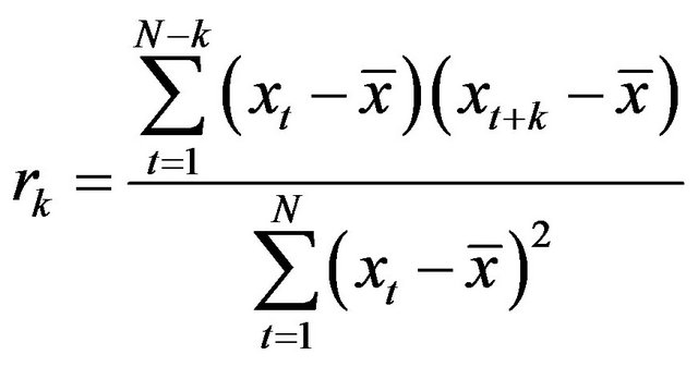
If the first observation in each pair is considered as the first variable and the second observation as the second variable [21], Equation (2) will be obtained which represents the autocorrelation between the observations with k distance [22].
 (2)
(2)
For the interpretation of autocorrelation, “autocorrelogram” is used in which autocorrelation coefficient is drawn against lags (lags). Although interpretation of this diagram is not easy, the following general states can be considered in this respect. If a time series is completely random, for large amounts of N and all non-zero values of k, the value of autocorrelation coefficient is equal to zero . Static time series often show short term correlation in which a relatively large amount of r1 with two or three time series, significantly greater than zero, consecutively get smaller and for longer lags, rk values tends to zero. If a time series on two sides of the mean tends to sequence, correlogram will tend to sequence as well, and if a time series has a trend, rk values do not drop, except for very large values of lag. From this correlogram cannot be much inferred since other aspects are surrounded by trend [20]. Correlogram represents a time series with seasonal changes (fluctuation in the same frequency). If correlogram in these series is drawn after elimination of seasonal change from data, we are provided with more information. With regard to time series and outlying observations, first, the outliers should be adjusted and then correlogram can be drawn so as it won’t be affected by these outliers. In addition, by correlogram and series partial correlogram, Order ARIMA Model [23] or the series randomness is determined. In this study, the data randomness was examined by calculation of autocorrelation and drawing correlograms.
3.2. Cross-Correlation
In case observations of two time series are available and the relationship between them is to be found, two states can be distinguished. In the first state, two series occur in “equal condition” the correlation of which is to be found. In the second case, which is more important, two series are “randomly correlated” so as one series is regarded as the input of a linear system and another series as the output [20]. In this research, precipitation time series of the two bases are in similar condition. Equation (3) is for calculation of cross-correlation between the two times series.
 (3)
(3)
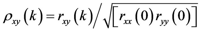
This function measures correlation between X(t) and Y(t+k). In the Equation (3), cross-correlation is calculated through covariance of the series. The symbols used in the equation are as follows:
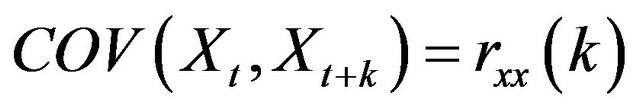 (4-1)
(4-1)
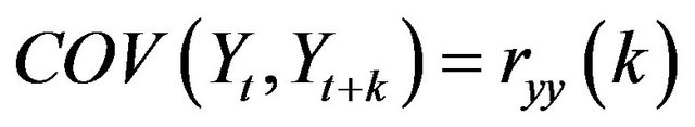 (4-2)
(4-2)
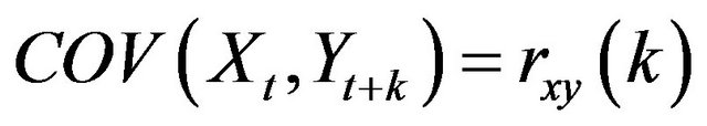 (4-3)
(4-3)
[20]. Application of cross-correlation is not recommended for the condition in which two time series do not follow an identical trend, since it may produce undesirable results.
3.3. Wilcoxon Test
To compare the mean of two time series, numerous parametric and non-parametric techniques can be employed if the required conditions are met. In cases where data do not meet the condition for performance of parametric tests, equivalent non-parametric tests can be applied. The quantile-quantile plot indicates that the data do not have a normal distribution. Hence, Wilcoxon non-parametric test which is equivalent to the two-sample parametric t-test was used which is a good substitute to it in case t-test conditions are not met. Mathematical form of this test, like t-test with a paired sample (correlated) is as the following Equation (3).
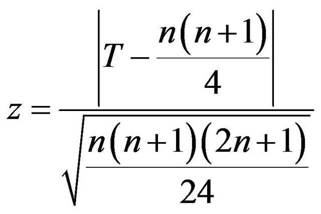 (5)
(5)
This test examines both direction and degree of difference between peer groups. Therefore, it answers the question as which part of pairs is greater than other and ranks the differences in the order of their absolute value, i.e. by means of this test it can be judged what part is greater than the other [24].
4. Research Findings
4.1. Study of Time Series Autocorrelation
Autocorrelation of the annual time series in none of the lags outside the upper and lower limit is significant and the amount of autocorrelation can be supposed equal to zero so as randomness of the annual time series can be confirmed, although APHRODITE time series is closer to a perfect randomness (Figures 1 and 2).
Table 1 provides the results of autocorrelation application for a month lag in the monthly time series and a season lag for the seasonal time series. The autocorrelation close to zero is confirmed in the monthly time series of April-May, September-October, October-November, January-February, February-March, and in the seasonal time series of spring and autumn. In other time series, autocorrelation in the mentioned lags is significant in the table. The time series of July-August lies farthest from the condition of a random time series. In addition, autocorrelation coefficient estimation indicates two points: first, in none of the monthly and seasonal time series there is a significant autocorrelation coefficient. Secondly, despite the difference in value of autocorrelation coefficient in some time series of the databases, the amount of this difference is trivial and statistically insignificant and the monthly and seasonal precipitation time series of the two databases have an identical autocorrelation in the month and season lags. After interpreting figures in Table 1, it can be claimed that in March-April time series in both bases indicate autocorrelation of precipitation in MarchApril 5 and 15 years before and after, whereas in the time series of April-May, the precipitation is not significant in any lag. In other words, April-May precipitation has no significant correlation with April-May precipitation the years before and after.
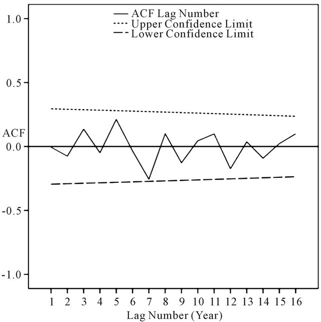
Figure 1. Correlogram database APHRODITE in the lag year.
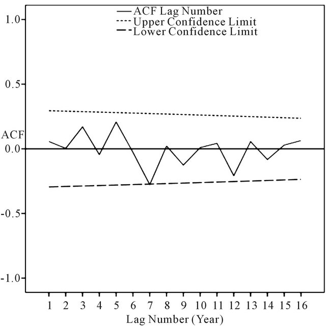
Figure 2. Correlogram database Asfazari in the lag year.
Table 1. Time series autocorrelation significance in the month lag for the monthly time series and the season lag for seasonal time series.
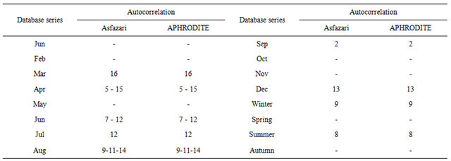
-: Signal to autocorrelation insignificance.
4.2. Studying Time Series Cross-Correlation Fluctuation Patterns
In Figure 3, the cross-correlation between the annual time series of APHRODITE and Asfazari databases indicates that correlation between the two series is significant in zero lag, i.e. maximum value of the cross-correlation in zero lag signifies simultaneity of the two series’ fluctuation peak [25], and as expected, despite the difference in precipitation estimation value, since the two bases represent one area, they have simultaneous peak and fall. For the monthly and seasonal time series, cross-correlation between time series of the two bases is significant in zero lag, indicating simultaneous peak and fall of monthly and seasonal time series. Only March-April and AugustSeptember time series have different situation so as in March-April time series, in addition to significance of cross-correlation in zero lag, cross-correlation in +5 and −5 lag is significant as well (Figure 4). In other words, the precipitation peak in March-April occurs with 5 days after and before. And in August-September time series, in addition to significance of cross-correlation in zero lag, cross-correlation in +2 and −2 lag is significant as well (Figure 5).
4.3. Means Difference Significance Test
In quantile-quantile plot, in low precipitation quantities, the observed precipitation in both bases is less than the expected normal precipitation. In APHRODITE data along with increasing precipitation, the observed and normal precipitation get closer to each other (Figure 6), whereas within the same area, the observed Asfarazi precipitation is higher than the expected normal quantity (Figure 7), and in high precipitation quantities, in both bases, the observed amounts are less than the expected normal precipitation. However, in APHRODITE base, the
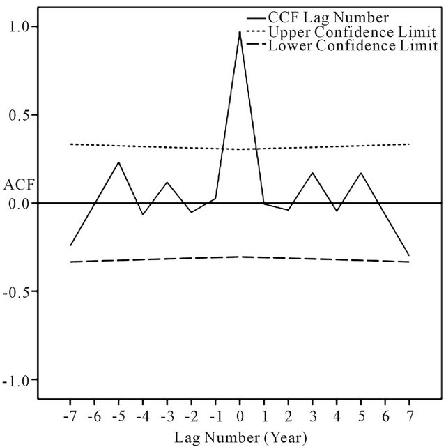
Figure 3. Cross-correlation between precipitation data of APHRODITE and Asfazari databases in year lag.
difference between the observed and expected precipitation is greater. Considering that application of the parametric tests by time series did not meet the required conditions, Wilcoxon non-parametric test was used as compared with the means, in which the null hypothesis suggests “there is no difference between the means of the two time series’ data” and the alternative hypothesis proposes “there is a difference between the means of the two time series’ data”. Based on the results, since the number and the mean of Asfazari ranks (positive) are greater than the number and the mean of APHRODITE ranks (negative), the mean Asfazari precipitation is greater than the mean of APHRODITE precipitation. This led to a negative value for Z-test statistic based on which at 0.05 chance of error
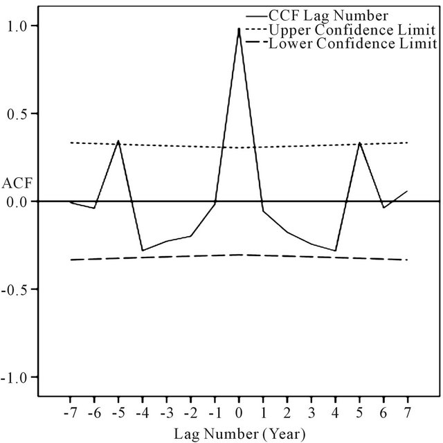
Figure 4. Time series cross-correlation in APHRODITE and Asfazari databases in month lag (April).
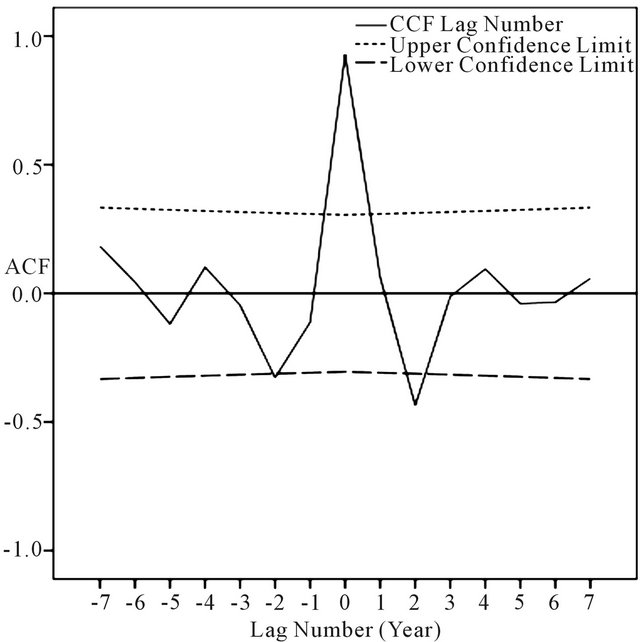
Figure 5. Time series cross-correlation in APHRODITE and Asfazari databases in month lag (September).
there is no sufficient reason to confirm the null hypothesis and at 95% confidence interval the difference between the mean precipitation of Asfarazi and APHRODITE is statistically significant and the alternative hypothesis is confirmed (Table 2).
The results of Wilcoxon test for the data’s mean in the monthly and seasonal time series are similar to those obtained from the test of annual time series. In the time series of March-April, May-June, July-August, AugustSeptember and December-January, although the value of
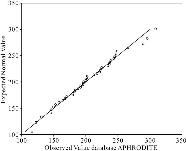
Figure 6. Normal Q-Q plot of annual precipitation of APHRODITE database.
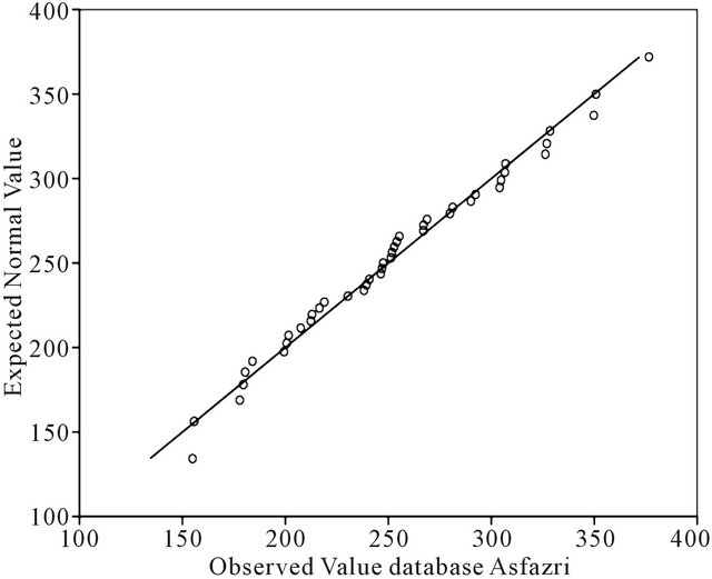
Figure 7. Normal Q-Q plot of annual precipitation of Asfazari database.
Table 2. Wilcoxon ranks and sign test of APHRODITEAsfarazi annual precipitation.
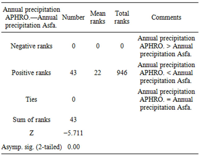
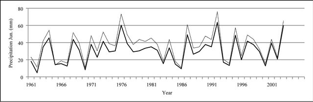
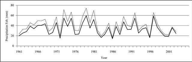
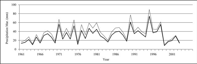
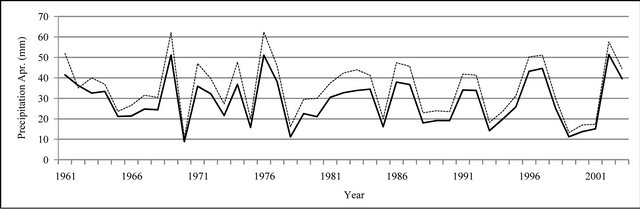
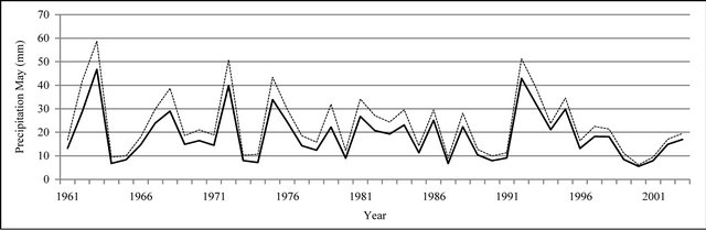
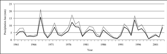
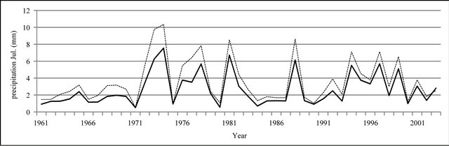
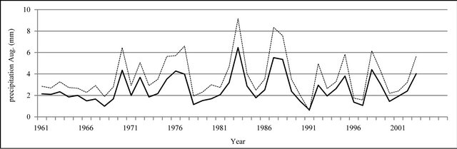
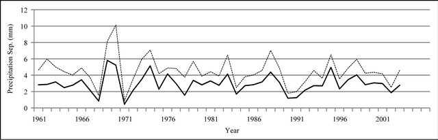
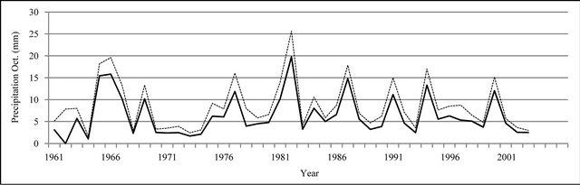
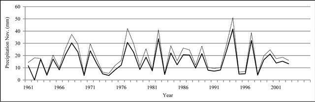
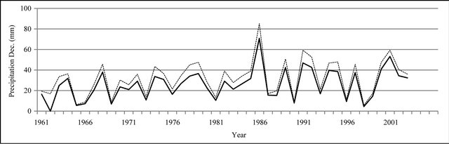
Figure 8. Monthly precipitation time series plot (mm).
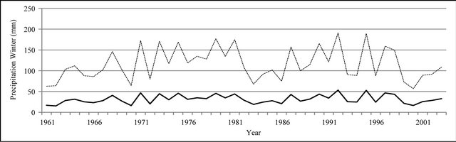
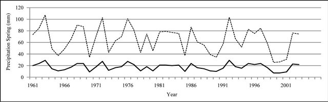
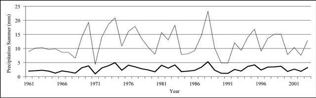
Figure 9. Seasonal precipitation time series plot (mm).
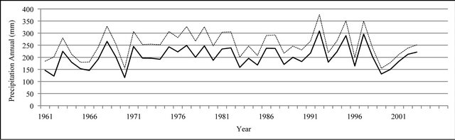
Figure 10. Annual precipitation time series (mm).
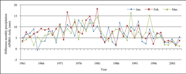
Figure 11. Difference of monthly precipitation time series database APHRODITE and Asfazari (mm).
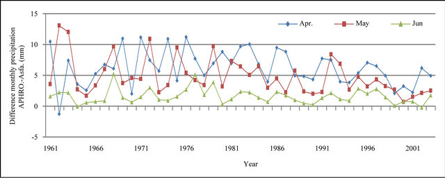
Figure 12. Difference of monthly precipitation time series of APHRODITE and Asfazari databases (mm).
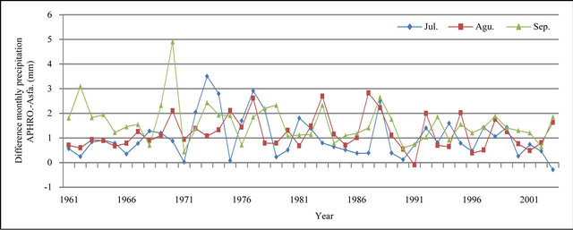
Figure 13. Difference of monthly precipitation time series of APHRODITE and Asfazari databases (mm).
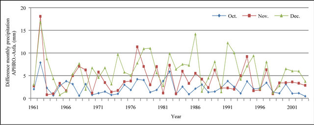
Figure 14. Difference of monthly precipitation time series of APHRODITE and Asfazari databases (mm).
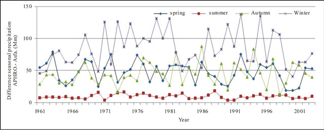
Figure 15. Difference of seasonal precipitation time series of APHRODITE and Asfazari databases (mm).
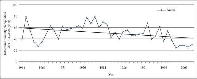
Figure 16. Difference of annual precipitation time series of APHRODITE and Asfazari databases (mm).
the test statistic somewhat becomes smaller, this drop in value is not statistically significant and still the mean difference of the time series is significant. In the time series of April-May, August-September, September-October, October-November, November-December, January-February and February-March and all the seasonal series, the negative ranks become zero. In these series, mean Asfarazi precipitation is greater than mean APHRODITE precipitation. In the monthly time series of March-April, May-June, July-August, August-September and December-January, the means of negative ranks are 1, 2.5, 7, 1 and 1, respectively. In other words, in these time series, there are cases where the mean monthly precipitation of APHRODITE is greater than that of Asfarazi.
4.4. Comparison of Time Series Plots
In Figures 8 to 10, APHRODITE time series are represented with continuous line and those of Asfarazi with dotted line at three monthly, seasonal and annual levels. The estimated precipitation quantity of Asfarazi base is greater than that of APHRODITE base. However, in March 1962, May 1964, 2002, June 2003, July 1991 and December 1965, precipitation quantity of APHRODITE base is found to be greater than that of Asfarazi, but this difference is so insignificant that even in the maximum case it reaches 1.3 mm which can be ignored. Yet, fluctuation in both series plots follows an almost similar pattern indicating an identical trend in them. The zero precipitation on APHRODITE base in three months of September-October, October-November and November-December of 1962 seems abnormal for which no data construction took place for explanation of precipitation features based on the data of this base. In Figures 11 to 16 respectively the difference of APHRODITE monthly (in 3 figures), seasonal and annual precipitation time series from those of Asfarazi (accept a few dispensable cases) is positive. In other words, precipitation quantity of Asfarazi base is greater than that of APHRODITE base but does not follow a particular pattern and is not regular and has fluctuations. For example, while precipitation difference of the two bases reaches 18 mm in January 2001, in January of the next year this difference decreases to 5 mm and in 2002 this difference becomes the least (1.5 mm). In general, the monthly and seasonal time series have decreased in recent decades. Yet, this is a general conclusion and some fluctuation cases can be noticed as well. Maximum difference between annual precipitation of the two bases is observed in 1962 (79 mm), minimum difference in 1999 (24 mm) and average difference is 50 mm. Comparison of the annual data difference indicates a decreasing trend in the difference between the two bases in recent years which most probably is due to the increase in number of the used gauging stations in APHRODITE bases.
5. Conclusions
Despite availability of diverse qualitative assessment and control methods applied in data supply and processing centers, for many reasons these data may be erroneous and comparison of data from different bases is a suitable method in assessment of data’s reliability and accuracy.
In this study, the time series of APHRODITE and Asfarazi bases were compared. The research results indicate that the estimated precipitation quantity in the monthly, seasonal and annual time series of APHRODITE base (except a few monthly series with insignificant quantities) has been smaller than that of Asfarazi base. However, the amount of this difference has not been constant and has had fluctuation. The data of Asfarazi database which has used a greater number of gauging stations in interpolation are more valid compared to those of APHRODITE base. However, in such studies, long time period and data extending beyond Iran’s political borders are required so as this base can be used considering the lower estimation of precipitation data in the latter base.
The monthly, seasonal and annual time series in both bases show a random behavior and in the series with autocorrelation follow a similar pattern. Studying crosscorrelation between series of the two bases indicates a statistically significant lag in zero lag in the monthly, seasonal and annual series, confirming simultaneity of the peak and fall in the two series. Wilcoxon test at 95% confidence confirms significance of the mean difference between the two series, and there is no sufficient evidence to confirm the null hypothesis suggesting absence of a difference between the means of the two series.
Finally, it seems that narrowing difference among the estimates of the two bases in recent years is due to the greater number of gauging stations used by APHRODITE database.
REFERENCES
- B. Podobnik, D. F. Fu, H. E. Stanley and P. Ch. Ivanov, “Power-Law Auto-Correlated Stochastic Processes with Long-Range Cross-Correlations,” European Physical Journal B, Vol. 56, No. 1, 2007, pp. 47-52. doi:10.1140/epjb/e2007-00089-3
- J. Brommundt and A. Bardossy, “Spatial Correlation of Radar and Gauge Precipitation Data in High Temporal Resolution,” Advances in Geosciences, Vol. 10, 2007, pp. 103-109. doi:10.5194/adgeo-10-103-2007
- H. Li, S. H. Futch and J. P. Syvertsen, “Cross-Correlation Patterns of Air and Soil Temperatures, Precipitation and Diaprepes Abbreviatus Root Weevil in Citrus,” Pest Management Science, Vol. 63, No. 11, 2007, pp. 1116-1123. doi:10.1002/ps.1431
- F. Capodici, G. Ciraolo, G. La loggia, L. Liuzzo, L. V. Noto and M. T. Noto, “Time Series Analysis of Climate and Vegetation Variables in the ORETO Watershed (Sicily, Italy),” European Water23/24, 2008, pp. 133-145.
- J. Y. Lee and K. Lee, “Use of Hydrologic Time Series Data for Identification of Recharge Mechanism in a Fractured Bedrock Aquifer System,” Journal of Hydrology, Vol 229, No. 3-4, 2000, pp. 190-201. doi:10.1016/S0022-1694(00)00158-X
- A. Katimon and A. Khairi Abd Wahab, “Hydrological Analysis of a Drained Peat Basin Using Time Series Correlation and Cross-Correlation Functions,” Journal of Technology, Vol. 39B, 2003, pp. 63-74.
- P. Angelini, “Correlation and Spectral Analysis of Two Hydrogeological Systems in Central Italy,” Journal of Hydrological Sciences, Vol. 3, No. 42, 1997, pp. 425-438. doi:10.1080/02626669709492038
- S. Rehman, and A. H. Siddiqi, “Wavelet Based Correlation Coefficient of Time Series of Saudi Meteorological Data,” Chaos, Solitons and Fractals, Vol. 39, No. 4, 2009, pp. 1764-1789. doi:10.1016/j.chaos.2007.06.054
- P. M. Biron, A. G. Roy, F. Courschesne, W. H. Hendershot, B. Cote and J. Fyles, “The Effects of Antecedent Moisture Conditions on the Relationship of Hydrology to hydrochemistry in a Small Forested Watershed,” Hydrological Processes, Vol. 13, No. 11, 1999, pp. 1541-1555. doi:10.1002/(SICI)1099-1085(19990815)13:11<1541::AID-HYP832>3.0.CO;2-J
- H. Sun and M. Koch, “Case Study: Analysis and Forecasting of Salinity in Apalachicola Bay, Florida, Using Box-Jenkins ARIMA Models,” Journal of Hydraulic Engineering, Vol. 127, No. 9, 2001, pp. 718-727. doi:10.1061/(ASCE)0733-9429(2001)127:9(718)
- S. Javanmard, A. Yagagai, M. I. Nodzu, H. Kawamoto, J. B. Jamali, K. Kamiguchi and O. Arakawa, “Comparing High-Resolution Networked Precipitation Data with Satellite Precipitation Estimates of TRMM 3B42 over Iran,” Advances in Geosciences, Vol. 25, 2010, pp. 119-125. doi:10.5194/adgeo-25-119-2010
- M. Rajeevan and J. Bhate, “A High Resolution Daily Networked Precipitation Data Set (1971-2005) for Mesoscale Meteorological Studies,” Current Science, Vol. 96, No. 4, 2009, pp. 558-562.
- M. Rajeevan, J. Bhate, J. D. Kale and B. Lal, “High Resolution Daily Networked Precipitation Data for the Indian Region: Analysis of Break and Active Monsoon Spells,” Current Science, Vol. 91, 2006, pp. 296-306.
- A. Mishra, A. Yatagai, A. Hamada and R. M. Gairola, “Estimation of Precipitation over Asia by Combined Use of Gauge and Multi-Satellite Sensor Observations at Fine Scale,” 91St Annual AMS Meeting, 24 January 2011.
- A. Yatagai, K. Kamiguchi, O. Arakawa, A. Hammed, N. I. Yasutomi and A. Kitoh, “APHRODITE: Constructing a Long-Term Daily Networked Precipitation Dataset for Asia Based on a Dense Networked of Rain Gauges,” Bulletin of the American Meteorological Society, Vol. 93, No. 9, 2012, pp. 1401-1415. doi:10.1175/BAMS-D-11-00122.1
- P. Xie, A. Yatagai, M. Chen, T. Hayasaka, Y. Fukushima, C. Liu and Y. Song, “A Gauge-Based Analysis of Daily Precipitation over East Asia,” Journal of Hydrometeorology, Vol. 8, No. 3, 2007, pp. 607-626. doi:10.1175/JHM583.1
- A. Yatagai, O. Arakawa, K. Kamiguchi, H. Kawamoto, M. I. Nodzu and A. Hamada, “A 44-Year Daily Networked Precipitation Dataset for Asia Based on a Dense Networked of Rain Gauges,” Scientific Online Letters on the Atmosphere, Vol. 5, 2009, pp. 137-140. doi:10.2151/sola.2009-035
- http://www.chikyu.ac.jp/precip
- F. Rahimzade, “Statistical Methods in Meteorology and Climatology Researchers,” Tehran, Iran, 2011.
- C. Chatfield, “The Analysis of Time Series an Introduction,” Ferdowsi University of Mashhad Press, Iran, 2003.
- H. A. Niroumd and A. Bozorgnia, “The Analysis Time Series,” Payam Nour University Press, Tehran, 2008.
- J. D. Cryer, “Time Series Analysis,” Ferdowsi University of Mashhad Press, Iran, 2006.
- H. Asakereh, “ARIMA Modeling for Tabriz City Annual Temperature,” Geographical Research Quarterly Tone, Vol. 93, 2009, pp. 3-24.
- K. Habibpour and R. Safari, “Comprehensive Guide to SPSS Application,” Motafekkeran Publication, Tehran, 2009.
- M. Chitsazan, M. S. Mirzaee and R. Chinipardaz, “Zoning of Abkhan Plain in Shahr-e-Kord City Using Time Series Analysis,” Scientific Journal of Shahid Chamran University, No. 17, 2007, pp. 1-15.