Journal of Sensor Technology
Vol.2 No.3(2012), Article ID:22874,7 pages DOI:10.4236/jst.2012.23021
Lookup Table Hough Transform for Real Time Range Image Segmentation and Featureless Co-Registration
1Department of Geoscience and Remote Sensing, Delft University of Technology, Delft, Netherlands
2Department of Geomatics, University of Cape Town, Rondebosch, South Africa
Email: b.g.h.gorte@tudelft.nl, george.sithole@uct.ac.za
Received June 9, 2012; revised July 13, 2012; accepted August 15, 2012
Keywords: Range Camera; Range Image Segmentation; Hough Transform; Co-Registration
ABSTRACT
The paper addresses range image segmentation, particularly of data recorded by range cameras, such as the Microsoft Kinect and the Mesa Swissranger SR4000. These devices record range images at video frame rates and allow for acquisition of 3-dimensional measurement sequences that can be used for 3D reconstruction of indoor environments from moving platforms. The role of segmentation is twofold. First the necessary image co-registration can be based on corresponding segments, instead of corresponding point features (which is common practice currently). Secondly, the segments can be used during subsequent object modelling. By realisising that planar regions in disparity images can be modelled as linear functions of the image coordinates, having integer values for both domain and range, the paper introduces a lookup table based implementation of local Hough transform, allowing to obtain good segmentation results at high speeds.
1. Introduction
Segmentation of 3-dimensional point clouds is gaining popularity as new range sensors, such as the Microsoft Kinect game controller (Figure 1), which turn out to be suitable as 3D data acquisition devices, are available at prices in the EUR100 range. Another example of a 3D input device is the Mesa Swissranger SR4000, which is essentially a single CCD/CMOS chip plus a number of infrared LEDS. It could become affordable for many applications when mass produced.
An often-mentioned application for such consumerprice 3D sensors is SLAM (Simultaneous Localization and Mapping) for indoor use. The goal is to have a device move around in an indoor environment, either being controlled by an operator or mounted on a mobile robot, and to create a 3D model of the environment, while keeping track of the position of the device with respect to the model being created. For the work flow this means:

Figure 1. The Kinect device with (from left to right) laser projector, RGB camera, and NIR camera.
• A sequence of 3D recordings is acquired from a moving platform;
• Orientation and co-registration is done automatically;
• The recordings (or derived features/objects) are combined into a single model.
Recently a number of promising results made with Kinect appeared on Internet and to some lesser extend in scientific literature. Very attractive results are reported by [1-3]. Open source implementations of SLAM algorithms are downloadable from [2,4,5]. The approaches for co-registration are usually based on automatically finding correspondences between various recordings in the intensity or RGB images (Figure 2), which are recorded by range cameras simultanously with the 3D data (Figure 3). The corresponding 3D coordinates are then used as initial estimate for a 3D transformation, e.g. using ICP-based methods [1,6]. The model output of the above-mentioned algorithms consists mostly of pointclouds, in which results of many subsequent recordings are combined, or of a mesh which is created over the resulting pointcloud.
In the current paper we address segmentation of range camera recordings. The task of segmentation is to identify planar surfaces: in the envisaged result a recording is subdivided into uniquely labeled segments, each corresponding to a single planar surface in the scene. The goal of segmentation in our current perception is twofold:
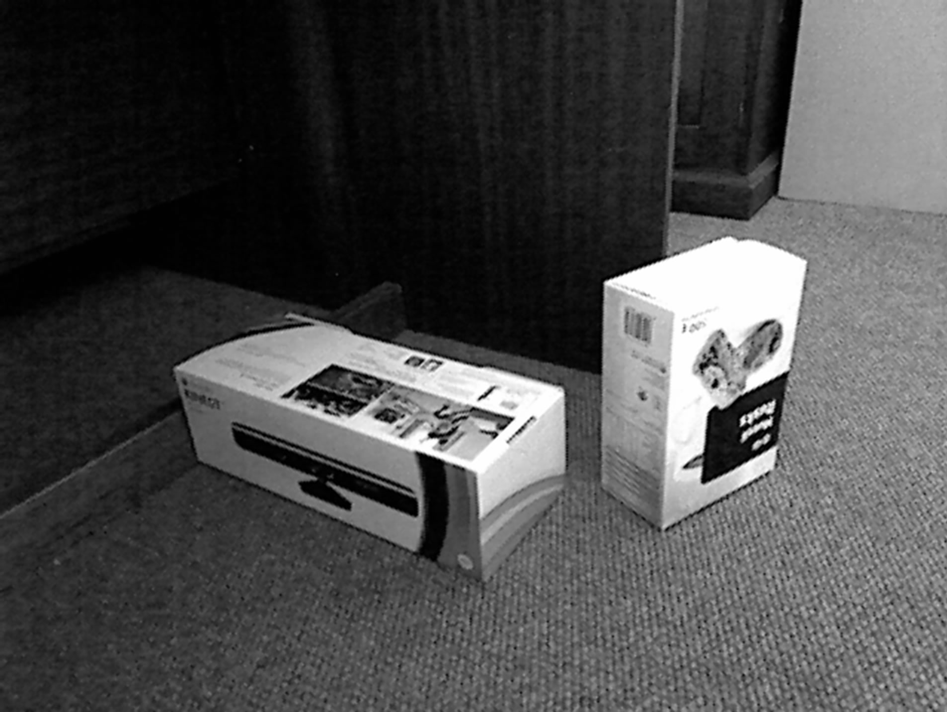
Figure 2. Kinect RGB image (green channel).
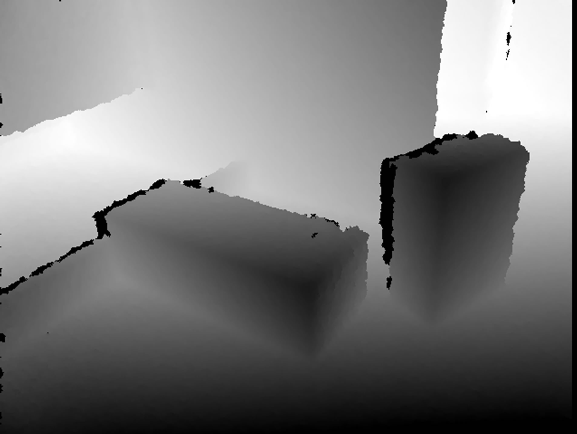
Figure 3. Kinect depth image.
First, we want to use the segmentation results for co-registration of the different images in the sequence. Instead of relying on corresponding points in different images (as first extracted from the RGB or intensity images and then combined with the range data), we want to use corresponding segments (i.e. planar surfaces). This will be elaborated in the remainder of the paper. Secondly, we want to use the segments during reconstruction of the 3D model. Ultimately, we are aiming at a model consisting of identified objects, rather than only of points. This will require not only segmentation, but also computation of surface boundaries and intersections etc.; however, this is a subject for further research.
The data used in the remainder of the paper have been acquired using a Microsoft Kinect. This device simultaneously records RGB and Range image sequences at video rate. The term range image implies a raster data structure (consisting of 480 × 640 pixels in this case), where each pixel value represents a measure of “range”, i.e. the distance between the camera and the observed object point in the scene (see also Section 2). Our goal is, therefore, range image segmentation rather than point cloud segmentation. This is a big advantage for real-time applications, because the problem is only 2.5D: to every (row, column) belongs only one range. Moreover, segmentation is about grouping of adjacent points belonging to the same planar surfaces, and in an image the adjacency relation (the fact that pixels are neighbors) is known beforehand, whereas in a point cloud the nearest neighbors of each point must be searched for explicitely.
As a limitation of the proposed method may be mentioned that it only segments according to planar surfaces. A generalization to other types of parameterized surfaces is not foreseen. We consider this acceptable, especially as the Kinect is intended to be used indoors, where planar surfaces (walls, ceiling, floor, various type of furniture) are usually abundant. If curved and other non-flat surfaces are present, they will lead to very small (or even single-pixel) segments, which will be ignored during coregistration and will not influence the results.
2. Plane Segmentation
The goal of the paper is range image segmentation according to planar surfaces. Conceptually, after translating each range image pixel (at image positition (x, y) and having range value r) into an (X, Y, Z) point in object space (see for example Figure 4), a plane is defined by the plane equation . Plane segmention on the basis of a range image, therefore, consists of estimating plane parameters a, b and c for each pixel on the basis of a neighborhood around the pixel, followed by a grouping of adjacent pixels with the same (of similar) parameter values into segments.
In [7] we studied various methods of obtaining a, b and c estimates in a rasterized aerial LIDAR data set. We
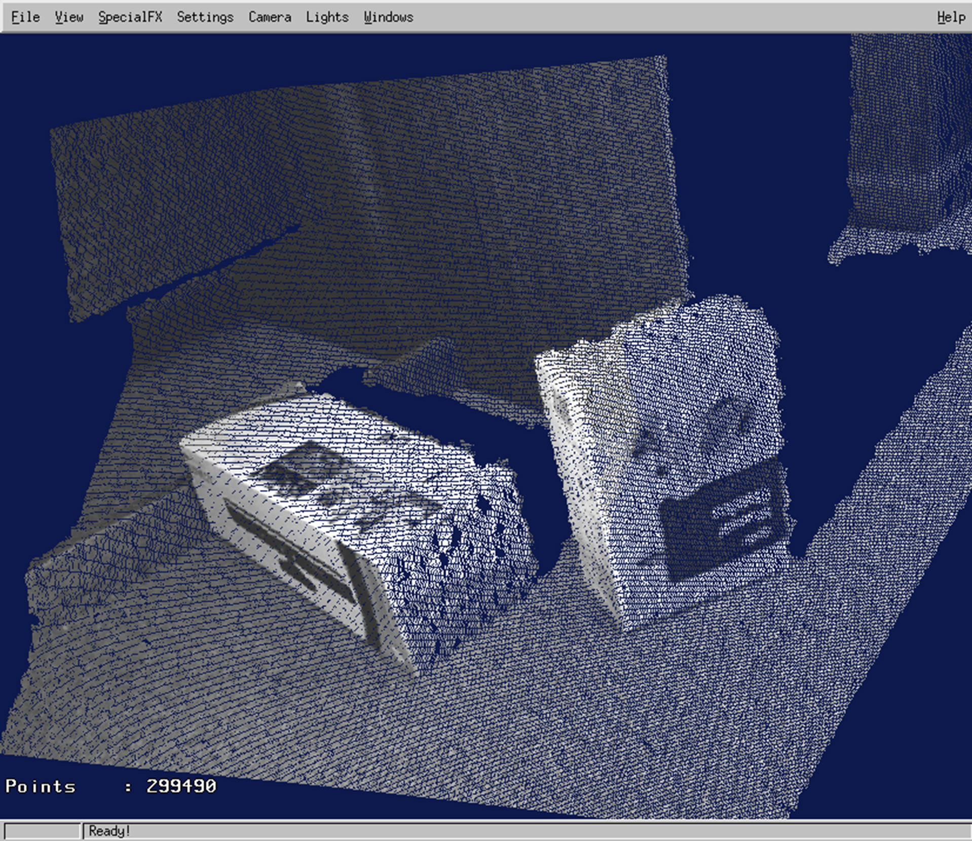
Figure 4. Point cloud generated by combining transformed range image with green channel of RGB image.
considered gradient and least squares approaches, and for both we introduced an improved, adaptive, variants, which resemble Nagao filtering: after identification of 5 subwindows at the center and the corners of the window under consideration, the plane parameters are taken from the “most planar” subwindow. Also we introduced a local Hough transform, which gave the best results—but at excessively high processing costs. In the current paper we briefly re-introduce local Hough transform for range camera data and present two optimizations in order to allow for real-time (video frame rate) performance.
2.1. Identifying Planes from Disparity
Kinect range image pixels represent disparity of a dot pattern, which is projected by a near-infrared (NIR) laser projector and recorded by a NIR camera (Figure 1). Because of the distance between projector and camera (of approximately 7.5 cm), the projected point pattern appears slightly shifted to the right in the camera images. Assuming that projector and camera are pointing parallel, the shift (called displacement) is always 7.5 cm in the object space. This translates into a number of pixels in image space. This number is called the disparity d and it depends on the depth Z to the object where the pattern is reflected (it also depends on the focal length f of the NIR camera expressed in pixels):
The working principle of the Kinect is based on the ability to measure this disparity in all elements of a 480 × 640 grid simultaneously, following a patented method.
The NIR camera resolution is in fact higher than the resulting range image: 1024 × 1280 instead of 480 × 640 pixels. Moreover, disparities are estimated “sub-pixel” and the (integer) values in the disparity image represent disparity with 1/8 pixel precision. Finally, instead of having/wdisparity = 0 at distance = infinity (as would be intuitive), an offset C is applied from which the observed disparity is subtracted in order to have the resulting Kinect values k increase with depth [8]. The relation is given by:
The values k are the pixel values in a raw Kinect depth image. The relation between these values and depth after calibrating for C is shown in Figure 5.
The afore-mentioned transformation from image space (x, y) and depth Z to object space (X, Y, Z) coordinates uses 
Figure 5. Depth vs. disparity.
and 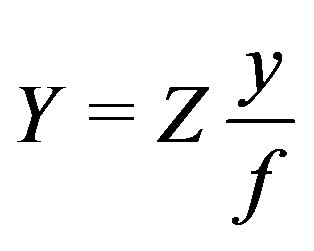 .
.
Since in a planar surface Z = aX + bY + c we get
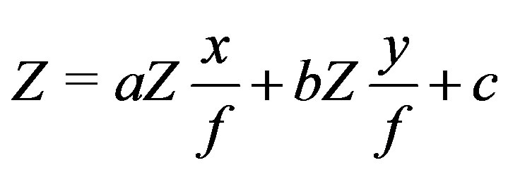
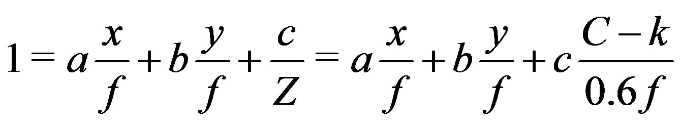
which can be re-arranged into: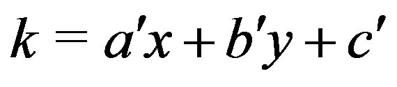
with ,
,  and
and .
.
This is a quite remarkable, however known, property of disparity [9]: A linear function Z(X, Y) in object space, i.e. a plane, is represented by a linear function k(x, y) in range image space. Planar surface segmentation can therefore be implemented as finding areas of adjacent pixels with the same (or similar) values for ,
,  , and
, and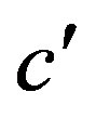 , based on the values and image coordinates of a disparity image. All of these are directly available from the device without any further computation. This is the basis for the first optimization.
2.2. Local Hough Transform
Hough transforms are a well-known class of image transforms [10], which have the purpose of idenfying parameterized objects of a certain class (be it a line, circle, plane, cylinder, sphere etc.). The principle is to construct for each pixel in the image that is a potential candidate for belonging to some object (of the class of interest), all possible combinations of parameter values such that an object with those parameters would indeed contain that pixel. An accumulator keeps track of the frequency in which the various combinations occur over the entire image and thereby builds up evidence for the existence of objects. Note that parameter values are assumed to be taken from a discrete sets, having a certain (limited) precision.
For example, having reconstructed a point (X0, Y0, Z0) from a range image, all planes satifying Z0 =aX0 + bY0 + c would contain that point. This leads to combinations of parameters (a, b, c) that can be found by choosing all possible (discrete) combinations of a and b, computing c = Z0 – aX0 – bY0 for each of them, and update the accumulator accordingly. When repeating this procedure for n points of which m ≤ n are in one plane, one would see the particular combination of (a, b, c) for that plane occuring m times.
Unfortunately, the practicality of a 3D Hough transform (with 3 parameters) is disputable because of high requirements to memory and processing capacity. In [7] we proposed a simplification that is more practicle, although still expensive. In this so-called local Hough transform we try to identify planar patches based on neighborhoods around each pixel (X0, Y0, Z0) in a range image, with the additional requirement that the pixel itself is part of the plane. We now reconstruct a plane Z – Z0 = a(X – X0) + b(Y – Y0) locally by inspecting the other pixels (X, Y, Z) in the neighborhood, constructing (a, b) combinations, storing these in a 2D accumulator and looking for the combination that occurs most often. This frequency of occurrence should equal the size of the window (minus one) if all points are coplanar, or be smaller if they are not. We hereby obtain an estimate for the a and b parameters (Figures 6 and 7) of the most likely plane containing the pixel, along with an indication of the likelihood of the plane. Note that the remaining plane parameter c at that pixel can be estimated as c = Z0 – aX0 – bY0 (Figure 8).
2.3. Lookup Tables
In the above paragraph we silently assumed to have (X, Y, Z) for each pixel available, whereas in reality they would have to be computed from disparity image coordinates (x, y) and values k. This is where we recall that planes in (X, Y, Z) are also planes in (x, y, k)—these values are directly available from the device. Moreover, x, y and k are integer numbers. If we take, for example, a window size of 7 × 7 pixels, (x – x0) and (y – y0) can only take values –3, –2, –1, 0, 1, 2, 3. Similarly, the range for (z – z0) might reasonably be limited to [–9..9]. Each of these 7 × 7 × 19 possibilities gives rise to a (discrete) number of (a’, b’) combinations, which can all be pre-computed and stored as a lookup table. This is the second optimization to local Hough transform base plane segmentation, as proposed in this paper.
3. Implementation
Range image segmentation is done in two steps:
• Estimation of plane parameters a, b, and c using Local Hough Lookup tables for each pixel, generating a, b and c image layers (Figures 6-8);
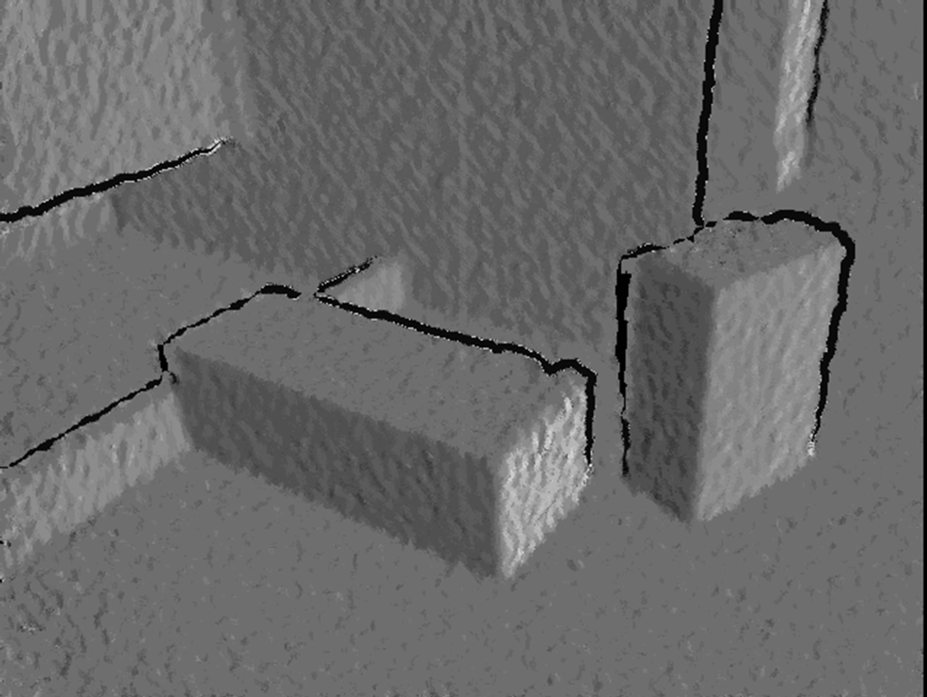
Figure 6. Estimated plane parameter a.
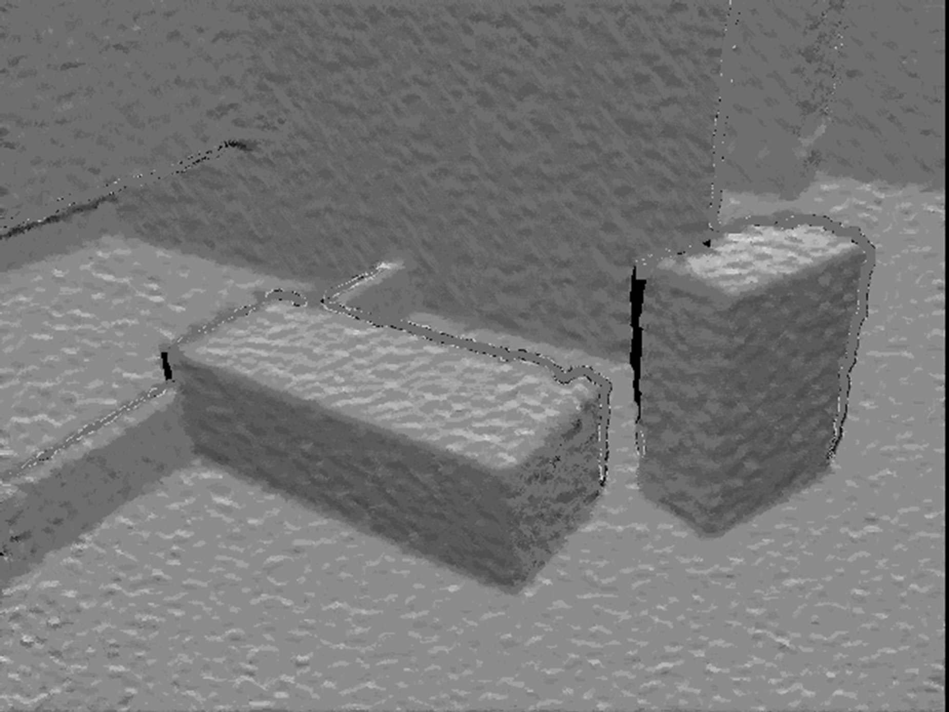
Figure 7. Estimated plane parameter b.
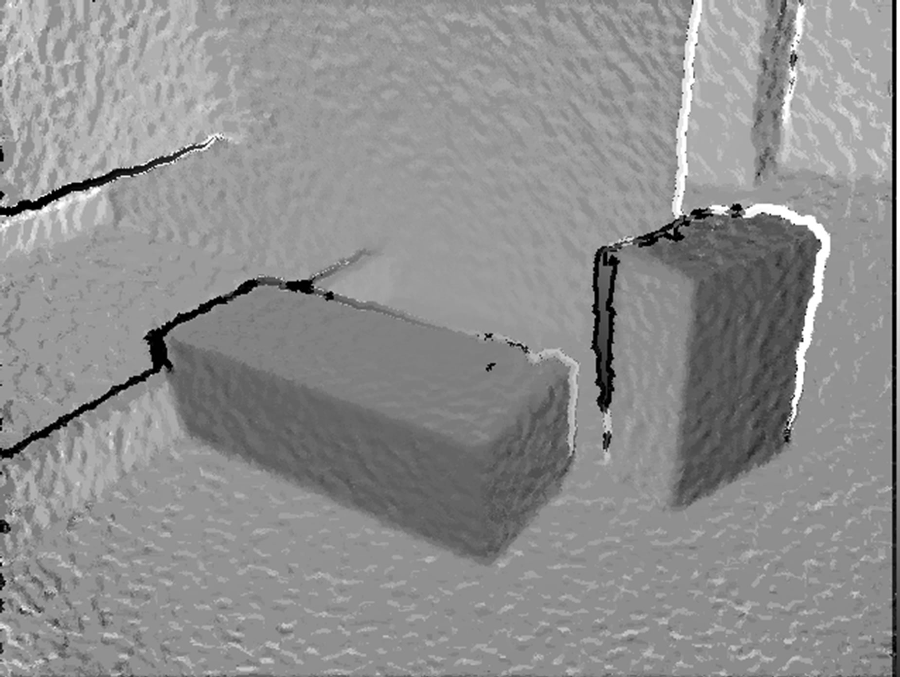
Figure 8. Estimated plane parameter c.
• Region merging: grouping of adjacent pixels with similar a, b, and c values into segments.
The implementation is descibed in the following two subsections.
3.1. Local Hough Lookup Tables
After a number of preliminary tests we have chosen to use for the local Hough transform parameter values as already mentioned in the description of the previous paragraph: a 7 × 7 window size and a range between –9 and 9 for the differences between the disparities of the central pixel and the surrounding pixels in the window. Furthermore, we have chosen ranges between –3 and +3 for the possible a and b values with a stepsize of 0.3. Therefore, a and b can take 21 different values each, with indices between –10 and 10. In order to avoid testing of the ranges, additional entries in the accumulator (with index values –11 and +11) are allocated to store any results that exceed the [–10 .. 10] range. These additional entries are not considered when determining the most frequent combination. The complete lookup table is, therefore, a 7 × 7 × 19 × 23 × 2 array. It should be regarded as a collection of 7 × 7 × 19 elements, each element being a 23 × 2 array. When processing a pixel within each 7 × 7 window the position (r, c) within the window (with respect to the central pixel) and its disparity d (relative to the central pixel) determine which of the 7 × 7 × 19 elements is selected. The selected element contains a set of 23 (a, b) combinations that are appropriate for that particular (r, c, d) combination.
LUT Initialisation
Before segmenting a Kinect range image sequence the lookup tables are set up, which means that for any valid combination of r, c and d the corresponding element is filled with 23(a, b) values that satisfy d = ar + bc. If  this is accomplished by having b run from –9 to 9 in steps of 1, and compute
 ; otherwise a runs from –9 to 9 and b is computed as
 . In both cases the results are rounded to the nearest integer before being stored in the lookup table.
LUT Usage
A pixel at row offset r (–3 ≤ r ≤ 3) and column offset c (–3 ≤ c ≤ 3) with respect to the central pixel, whose disparity differs by d (–9 ≤ d ≤ 9) from the one at the central pixel, selects the element [r + 3, c + 3, d + 9] from this lookup table. This yields a 23 × 2 array of (a, b) combinations that are supported by this (r, c, d). Each of the 23 pairs is an index pointing to a position at which the 2d accumulator array is incremented by one. This process is repeated 48 times: for each window element except the central one. Four examples of how the accumulator looks after these 48 iterations are shown in Figure 9. Subsequently it is determined at wich position in the accumulator array the maximum value occurs. This gives a (row, column) position in the array, and after subtracting (11, 11) (the index of the central position) and multiplying with the stepsize 0.3, the plane parameters a and b are known.
3.2. Region Merging
After extracting the a, b and c features for each pixel in the first step, the second step of segmentation is a process that groups adjacent pixels with similar feature values into segments. Various segmentation algorithms are descibed in recent and not-so-recent literature, such as region growing and clustering followed by connected component labeling. We are obtaining good results with a quadtree based region-merging algorithm [11]. The algorithm starts with treating each quadtree leaf as a candidate segment, followed by a recursive merging of adjacent leafs into subs-segments and sub-segments into segments. The process is controlled by two criteria: two adjacent segments are merged if and only if:
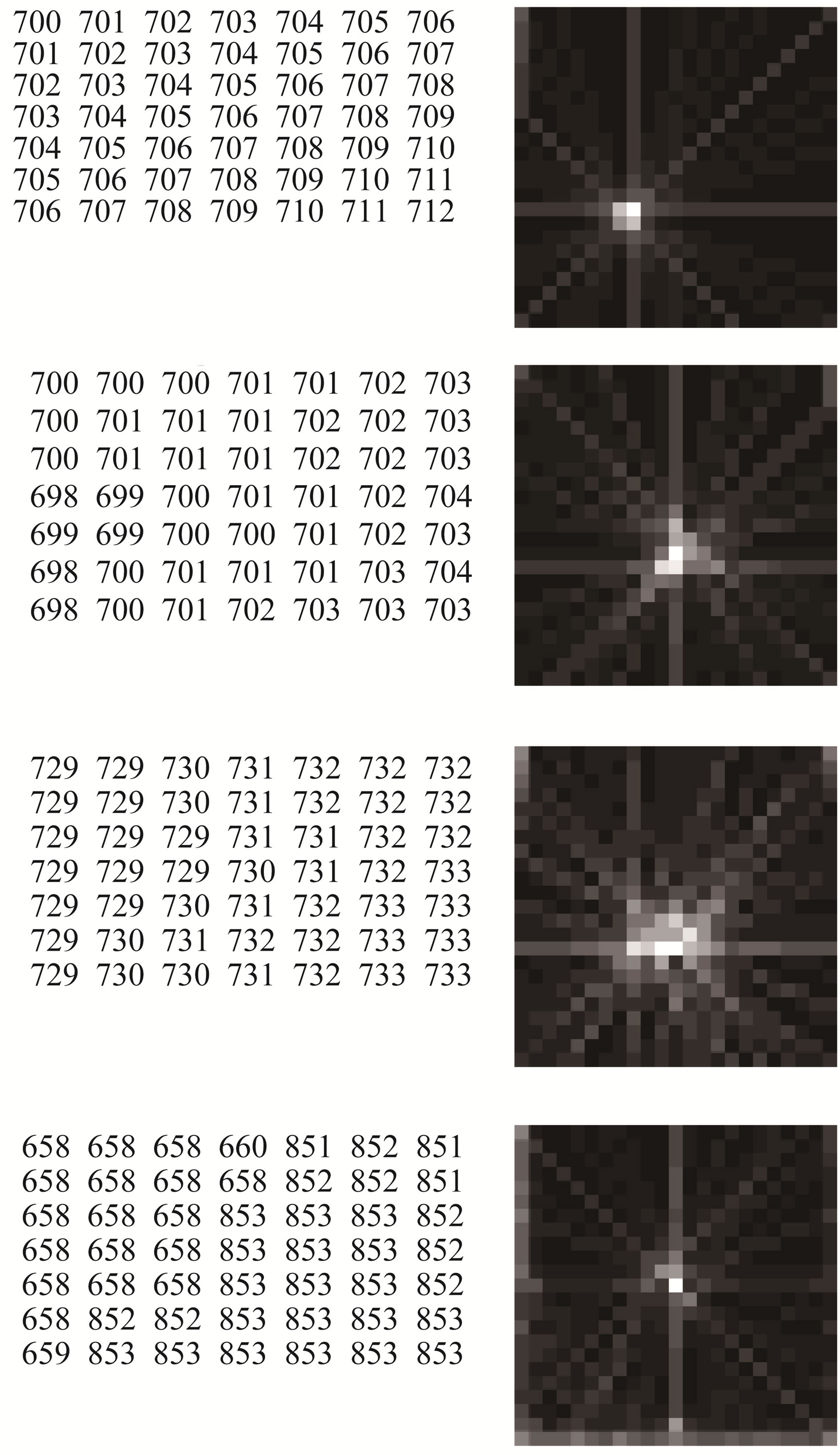
Figure 9. Examples of numerical disparity image fragments (left) and result accumulator arrays (right).
1) The mean values within the two segments do not differ more than a threshold T;
2) The variance in the resulting (merged) segment is less than T2.
As a result of this process segments with arbitrary shapes and sizes (in 2D) can be created, as long as the two above criteria continue to be satisfied. Note that in 3d the segments are expected to consist of co-planar pixels, however.
4. Results
Resulting a, b and c images are shown in Figures 6-8. These are input for region merging. The output is show in Figure 10.
Speed
An important consideration for the lookup table implementation of local Hough transform was the expected increase in speed, compared to the original version of [self reference]. Although the increase is remarkable indeed, it still does not fully comply with the real-time requirement that was set out in the beginning, as far as full-resolution (480 × 640) images are concerned. For images of those sizes, the entire process takes around 1.5 s, which is more or less equally divided over the feature extraction and the region merging phase.
The following remarks apply:
1) Kinect range images are acquired at a resolution of 480 × 640 pixels. However, the images show quite some autocorrelation, in addition to noise (see Figures 6-8). When sub-sampling the images to (say) a quarter of the resolution (120 × 160) not much information is lost, whereas noise is significantly reduced and segmentation is improved in terms of surface reconstruction accuracy;
2) Whereas the feature extraction phase was quite carefully optimized in the course of this study, the region merging phase was not optimized yet. It consist of a large
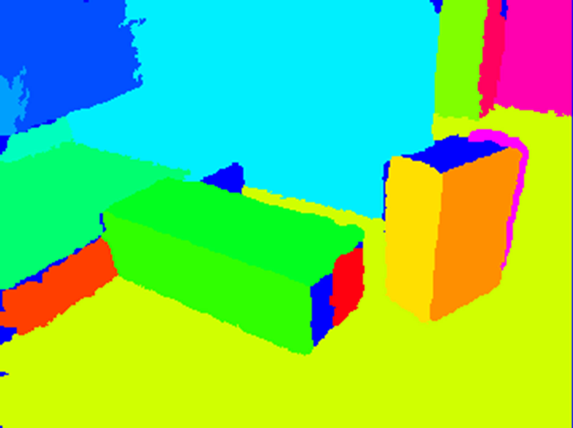
Figure 10. Segmentation result controlled.
number of steps, carried out by different executables passing image files between one and another as follows:
a) Exporting the a, b and c images into raster files;
b) Converting from raster to quadtree;
c) Overlaying a, b and c quadtrees into a combined one;
d) The actual segmentation;
e) Selecting significant (large enough) segments;
f) Converting from raster to quadtree files;
g) Filling small holes;
h) Importing the result for further processing (co-registration).
Futher optimisations, primarily by keeping the data in memory, can therefore be easily implemented.
3) The combined result of the above is expected to yield a more than 15-fold increase in frame rate (>10 fps), which might be sufficient for the envisaged application. If the maximum acquisition frequency of 30 fps should be reached, a faster computer is necessary—currenty a low-end laptop with an Intel dual core M450 processor at 2.40 GHz is used.
5. Application
Currently we are investigating how segmentation results can be used as a basis for performing co-registration of subsequent images in the sequence. The idea is to find corresponding segments, which is currently based on the expectation that at least a small overlap exists between corresponding segments, while the segment numbering is not necessarily the same in both images. In a cross table of all occuring segment combinations resulting from an overlay operation the valid combinations are selected on the basis of a and b values, such that these result in uniform (small) rotations over the entire image. After that the second image is translated and rotated such that an optimal fit of planes through corresponding segments is obtained.
Figure 11 shows three segmentation results of subsequent images of a simple scene with 6 planes, and two overlays of images 1 and 2, and 2 and 3 respectively. In Figure 12 a point cloud is shown that results from the
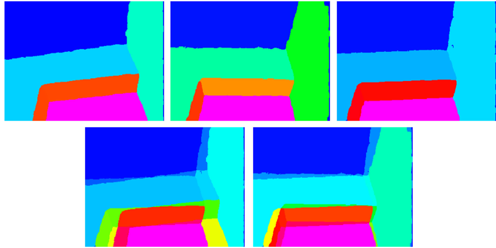
Figure 11. Above: segmentations of three subsequent images; below: overlays.
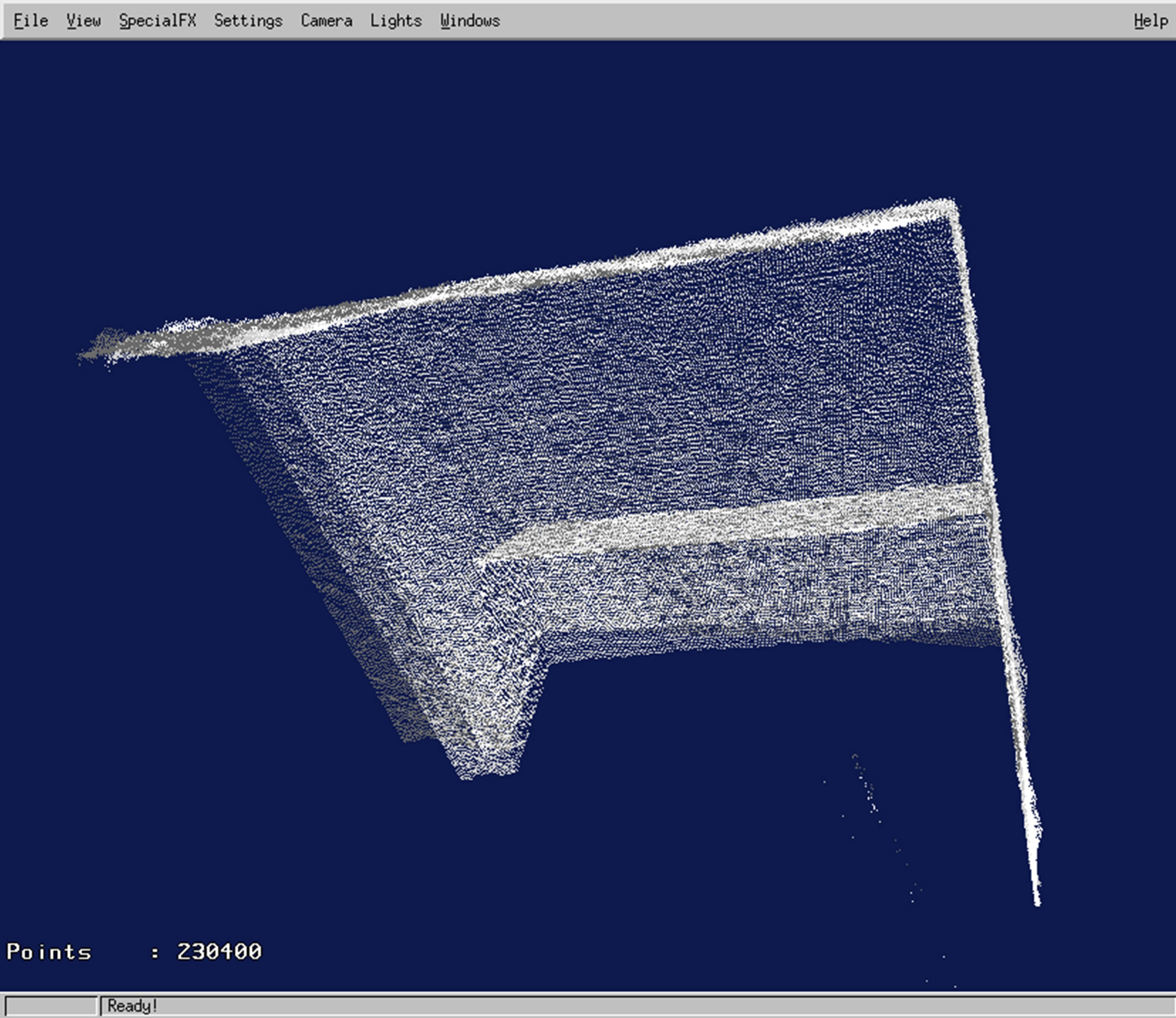
Figure 12. Point cloud after co-registration of three subsequent images.
three co-registered range images.
6. Conclusions
The paper presents an implementation for a local Hough transform of range images using lookup tables. This causes a very big increase in execution speed that almost reaches range camera accuisition speeds (in the order of 30 fps) if a 4-fold decrease of resolution is accepted.
We also have shown first results of range image coregistration using the segmentation result, which does not require any point correspondences as long as at least three intersecting planes can be identified. In case of fewer planes, a combination with point correspondences can still be a solution, but this has to be further investigated.
We believe those developments are important steps towards fully automatic real-time 3D modelling of indoor envirmonments using consumer-price range cameras.
REFERENCES
- P. Henry, M. Krainin, E. Herbst, X. Ren and D. Fox, “RGB-D Mapping: Using Kinect-Style Depth Cameras for Dense 3D Modeling of Indoor Environments,” International Journal of Robotic Research, Vol. 31, No. 5, 2012, pp. 647-663. doi:10.1177/0278364911434148
- N. Burrus, M. Abderrahim, J. G. Bueno and L. Moreno, “Object Reconstruction and Recognition Leveraging an RGB-D Camera,” Proceedings of the 12th IAPR Conference on Machine Vision Applications, Nara, 13-15 June 2011.
- S. Izadi, D. Kim, O. Hilliges, D. Molyneaux, R. Newcombe, P. Kohli, J. Shotton, S. Hodges, D. Freeman, A. Davison and A. Fitzgibbon, “KinectFusion: Real-Time 3D Reconstruction and Interaction Using a Moving Depth Camera,” 24th Annual ACM Symposium on User Interface Software and Technology, Santa Barbara, 16-19 October 2011.
- The OpenKinect Project, 1 June 2012. http://www.openkinect.org
- C. C. Stachniss, U. Frese and G. Grisetti, “OpenSLAM,” 1 June 2012. http://www.openslam.org
- S. Rusinkiewicz and M. Levoy, “Efficient Variants of the ICP Algorithm,” International Conference on 3-D Digital Imaging and Modeling, Quebec City, 28 May-1 June, 2001, pp. 145-152.
- B. Gorte, “Roof Plane Extraction in Gridded Digital Surface Models,” International Archives of Photogrammetry and Remote Sensing, Vol. 8, No. 2-3, 2009, pp. 1-6.
- K. Konolige and P. Mihelic, “Technical Description of Kinect Calibration,” 1 June 2012. http://www.ros.org/wiki/kinect_calibration/technical
- J. Weber and M. Atkin, “Further Results on the Use of Binocular Vision for Highway Driving,” SPIE Proceedings, Vol. 2902, 1997, pp. 52-61. doi:10.1117/12.267162
- P. V. C. Hough, “Method and Means for Recognizing Complex Patterns,” US Patent No. 30696541962.
- B. Gorte, “Probabilistic Segmentation of Remotely Sensed Images,” Ph.D. Thesis, ITC, Faculty of Geo-Information Science and Earth Observation, Enschede, 1998.