Journal of Signal and Information Processing
Vol.3 No.4(2012), Article ID:24974,11 pages DOI:10.4236/jsip.2012.34062
Comparing the Time-Deformation Method with the Fractional Fourier Transform in Filtering Non-Stationary Processes
![]()
1Statistics Genomics Unit, NIH/NIMH (National Institutes of Health/National Institute of Mental Health), Bethesda, USA; 2Department of Statistical Science, Southern Methodist University, Dallas, USA.
Email: mengyuantracy@hotmail.com
Received August 24th, 2012; revised September 26th, 2012; accepted October 6th, 2012
Keywords: Filtering; Time-Frequency; Time-Deformation; Fractional Fourier Transform
ABSTRACT
The classical linear filter is able to extract components from multi-component stochastic processes where the frequencies of components do not overlap over time, but fail for those processes where the frequencies overlap over time. In this paper, we discuss two filtering methods for non-stationary processes: the G-filtering method and the Fractional Fourier transform (FrFT) method. The FrFT method is mainly designed for linear chirp signals where the frequency is linearly changing with time. The G-filter can be used to filter signals with wide range of frequency behaviors such as linear chirps, quadratic chirps and other type of chirp signals with strong time-varying frequency behavior. If frequencies of the components can be approximated or separated by a straight line or a polynomial curve, the G-filter can successfully extract components from the original series. We show that the G-filter is applicable to a wider variety of filtering applications than methods such as the FrFT which require data of a specified frequency behavior.
1. Introduction
The traditional linear filter is defined as
 , where
  and
and , and
, and  and
and  are the input and output processes. A fundamental filtering result, see Papoulis (1965) [1] and Shumway and D. S. Stoffer (2000)
[2], is that , where
  and
and
 are the power spectra of stationary input and output processes
  and
and  respectively, and
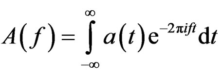 is the Fourier transform of
 .
.
This theorem illustrates how the linear filter affects the spectrum of the output processes. Based on this, certain linear filters, such as the Butterworth filter (Butterworth (1930) [3], have been designed to extract components from multicomponent time series, For a low-pass Butterworth filter,  , where
is the cutoff frequency, and N is the order of the filter. As N gets larger,  approximates a step function with domain
 . So, applying a low-pass Butterworth filter with an appropriate order N can filter the low frequency behavior below the cut-off frequency
 . The opposite applies to a high-pass Butterworth filter.
For stationary time series where the frequency stays constant over time, and for those non-stationary time series where the frequencies of different components do not overlap over time, the traditional linear filter with a single cut-off frequency can successfully extract components. But, for non-stationary time series with time varying frequency behavior (TVF), especially where the frequencies of components overlap over time, directly applying the traditional linear filter will not be able to extract components. (See Xu, Woodward and Gray (2012) [4].) Some non-linear filtering techniques can be used to address this issue such as the Fractional Fourier transform (FrFT) method, which has been widely used in signal processing especially to filter linear chirp signals. Xu, et al. (2012) [4] proposed the G-filtering method based on the time deformation method. This method can be widely used to filter a large range of different types of non-stationary signals with multiple frequency structures. The objective of this paper is to compare the two methods for filtering signals with different types of time varying frequency behaviors (TVF).
This paper is organized as follows. In Section 2, we review the time-deformation method. In Section 3, we review the FrFT method. In Section 4, we report the results of comparison studies which compare these two methods by filtering different types of data with TVF.
2. The G-Filter or the Time Deformation Method
The G-filter or the time deformation method is based on the concept of transforming the frequency behavior of the data by deforming the time scale. If viewed from the frequency domain point of view, rather than applying a constant cut-off frequency as in the traditional linear filter, the G-filter applies a time-dependent cut-off frequency function to filter components. Below we review the basic concept and definition of the G-filter.
Definition 2.1: A process  is called a dual of a stochastic process
  if there exists a mapping
  of which a well-defined inverse function
 exists so that
 when
when . The mapping
 is called the time-deformation function.
Definition 2.2: A process  is a Gstationary process if and only if a stationary dual process
  exists under some time-deformation function
 .
.
The earlier work by Gray, Vijverberg, and Woodward (2005) [5] focused on the transformation 
 . Jiang, Gray and Woodward (2006) [6] used the Box-Cox transformation
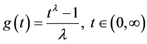 which is called a
  transformation. (
 transformation uses a parameter called offset to describe the sample origin.) Liu (2004) [7] and Robertson, Gray, and Woodward (2010) [8], considered the linear chirp transformation
 . These time-deformation procedures are available in the GWS software written in S+, which is downloadable from the website http://www.texasoft.com/atsa. While these authors used time transformations for purposes of producing a stationary time series in the dual space, our primary goal in this paper will be to find a time transformation to produce dual data from which the components can be separated in the frequency domain.
If a stochastic process  is G-stationary under some time deformation function,
  , Jiang, et al (2006) [6] proved that the generalized instantaneous frequency is approximately proportional to
 . Boashash (1992) [9] has shown that if a component has a phase function
 , then the instantaneous frequency is
 . Thus for the G-stationary process,
  , this time-deformation function
  is approximately proportional to its phase function
 .
.
Suppose the phase function of a signal is . Let
. Let  be a monotonic time deformation function. Then in the dual space, the phase function becomes
  and the instantaneous frequency becomes
 . For a process consisting of two components, one with a phase function
  and the other
 , the instantaneous frequencies of these two components are
  and
and . In the dual space, they are
  and
and
 .
.
If then
then . Or, in the dual space, the two components can be extracted by the traditional linear filter with a constant cut-off frequency if these two components can be separated by some G-stationary component (viewed in the frequency domain) in the original space. This leads to the definition of the G-filter.
Definition 2.3: Given a stochastic process
 and an impulse response function,
 , the G-filter or G-convolution is defined as
 where
where  is the usual convolution, and
 and
and ,
,
 , are the duals of
  and
and  under the time-deformation function
 .
.
Applying the principle of unitary equivalence systems (Baraniuk and Jones (1995) [10]), the G-filtering procedure has the following steps: 1) take an appropriate time deformation,  , on the original data to obtain a dual process that does not have overlapping frequencies in the frequency domain (which can be shown in a Wigner-Ville time frequency plot (Boashash (1992)) [9]; 2) apply the traditional linear filter on the dual process to extract components; 3) transform the filtered dual components back to the original time scale.
For a process consisting of two or more components, there are two ways to find a time-deformation function so that in the dual space the frequencies do not overlap over time and the components are separable. One is to treat one of the components as G-stationary and find a time deformation to transform this component into stationarity. Such a time deformation is based on the exact frequency behavior of one of the components. The other involves finding a time deformation function  such that
  and making the time-deformation based on
 . Here, the time-deformation only partly depends on the original components’ frequency behavior and there can be multiple choices of such a time-deformation function. (See Xu, Woodward, Gray (2012) [11]).
In the following example, we utilize the G-filter to filter a stochastic process consisting of two linear chirp components with TVF.
Example 2.1:
A realization from this process is displayed in Figure 1(a). The instantaneous frequencies of the two components are linearly changing with time as is illustrated in the Wigner-Ville time-frequency distribution in Figure 1(b). Such signals are called linear chirps and are of particular interest in acoustical and optical systems. Notice that the frequency level of the low frequency component after time t = 3 is similar to that of the high frequency component before time t = 1. For this type of data, the traditional filters fail to extract components, since they do not properly account for the time-varying frequency behavior, or they do not adjust the cutoff frequency with time according to the frequency behavior of the data.
Here, we use the time deformation method to filter each component. First, an appropriate time deformation function needs to be chosen. Observing that the high and low frequency components can be separated by a cut-off frequency, 0.06, up to time 2, we use a high-pass Butterworth filter with this cut-off frequency to obtain a front piece of the high frequency component. From this piece of data, GWS chooses a G(λ) time-deformation
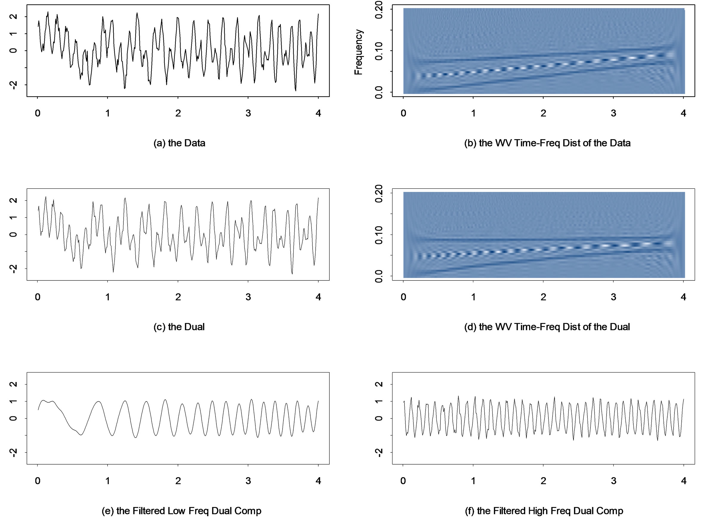
Figure 1. (a) and (b) A realization and its Wigner-Ville time-frequency distribution; (c) and (d) The dual data and its Wigner-Ville time-frequency distribution; (e) and (f) The two filtered dual components.
with λ = 1.3 and offset = 147, which can approximately stabilize the frequency level of the high frequency component as illustrated in Figure 1(d). These two dual frequencies do not overlap over time as compared with the original frequencies shown in Figure 1(b). Now, a Butterworth filter with a cut-off frequency 0.0725, is applied to the dual data so that the two components in the dual space are extracted, which are then transformed back into the original time scale by reinterpolation (See Xu, et al. (2012) [11]). The results (Figure 2) suggest that the time deformation method has successfully extracted both components from the original data.
3. The Fractional Fourier Transform
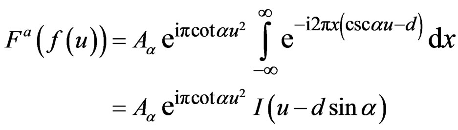
The fractional Fourier transform (FrFT) is a generalization of the classical Fourier transform. It is a valuable tool for the analysis of the linear chirp signals. The ath order FrFT is a linear operator defined by the integral (Ozaktas, Zalevsky and Kutay (2000) [12]).
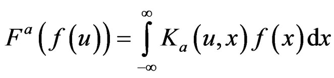 , (4)
, (4)
where

and 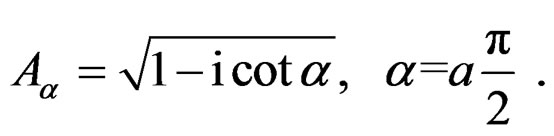
The FrFT is a powerful tool for filtering linear chirp signals. For a complex linear chirp signal
 ,
,
 . (5)
. (5)
When  or
or ,
,
 . (6)
. (6)
Here,  is the Dirac delta function or
  when
when  and
and  when
when .
.
Or the FrFT with order 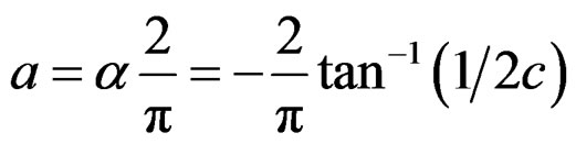
transforms a complex linear chirp signal into a Dirac

Figure 2. (a) and (b) THe two recovered components; (c) and (d) The two real components; (e) and (f) The Wigner-Ville time-frequency distribution of the two recovered components.
delta function. A real valued linear chirp signal consists of two complex conjugate signals which can be transformed into Dirac delta functions at order
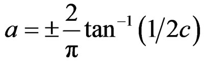 . For a sampled signal, these orders are given by
  (Capus and Brown
(2003) [13] and Ozaktas, Arikan, Kutay, and Bozdagt (1996) [14]), where  is the sampling frequency and N is the number of samples. For example, take a sample of
  on
on  with a sampling rate 100 points per time unit, then at the orders
 , the two complex components will be transformed into two approximations of Dirac delta functions.
The FrFT is a linear operator with the additive property,  and
and
 ,
,  , for any functions
 ,
, and
and . Thus
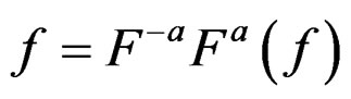 . If
. If  is known,
  can be recovered by applying an inverse FrFT with order “a” (Ozaktas, et al. (2000) [12]).
In order to extract a complex valued linear chirp signal, use of the FrFT involves first finding the order “a” at which the FrFT can transform this signal into a Dirac delta function, then masking out this Dirac delta function and transforming the remaining part back into the original space using the inverse FrFT. For a real valued chirp signal consisting of two complex components, two FrFT steps for each compon ent are needed to filter out the chirp signal (See Ozaktas, et al. (2000) [12]). Note that masking out a Dirac delta function means to zero out those values in the peak region which are not zero.
Example 3.1:

This is the same example as Example 2.1. As discussed above, the two FrFT orders for each component can be calculated as 0.97 and 0.95. If the underlying model is unknown, these orders are typically found by searching over the possible values of the order of the FrFT on (0,1) to see which order can generate an output with a high peak or a Dirac delta function (Ozarkas, et al. (2000) [12]). The filtering steps are: 1) Apply the FrFT with order a = 0.97(0.95) to the original data; 2) Mask out the peak in the output of step 1); 3) Apply the FrFT with order a = –0.97 × 2 (–0.95 × 2) to the output from previous step; 4) Mask out the peak in the output of the previous step; 5) Apply the FrFT with order a = 0.97(0.95) to recover the low (high) frequency component. This procedure is illustrated in Figure 3. The results are given in Figure 4, which show that the FrFT method has successfully extracted each component.

Figure 3. The FrFT filtering procedure for recovering the low frequency component of Example 3.1: (a) The original data; (b) Applying a FrFT with order 0.97 to the original data; (c) Masking out the peak in (b); (d) Applying a FrFT with order −0.97 × 2 to the output shown in (c); (e) Masking out the peak in (d); (f) Applying a FrFT with order 0.97 to the output shown in (e).
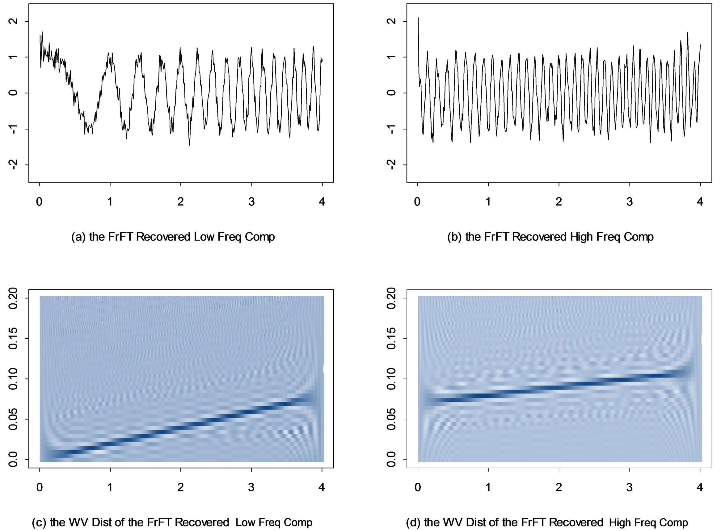
Figure 4. (a) and (b) The recovered low and high frequency components from the FrFT; (c) and (d) the Wigner-Ville timefrequency distribution of the two recovered components.
4. Comparing the G-Filter and the FrFT in Filtering Non-Stationary Processes
In the previous two sections, we have illustrated the methodology of the G-filter and the FrFT methods in filtering non-stationary processes, in particular, linear chirp processes whose instantaneous frequency exhibits a linear change with time. Some bat echolocation data and whale data consists of multiple linear chirp signals and have show linearly changing frequency behavior. Other types of data with time varying frequency behavior include quadratic chirps, cubic chirps, etc, of which the instantaneous frequencies of components are changing with time as a quadratic or cubic curve. Examples 2.1 and 3.1 have shown that both methods can successfully extract linear chirp signals from the original data. In this section, we mainly compare the FrFT and the G-filter for filtering the TVF components whose frequency change behavior is not linear. The first example will be to filter out quadratic chirp components whose frequency change follows a quadratic curve in time; the second will be to filter out the M-stationary components (Gray, et al. (2005) [5]) whose frequency change is like 1/t and thus is even more different from linearity.
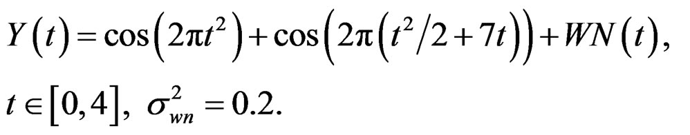
Example 4.1: Consider the process

where 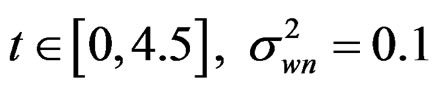
This process consists of two quadratic chirp components. The Wigner-Ville time-frequency distribution (Figure 5(d)) shows that the frequency behavior of the two components changes nonlinearly in time.
First we consider the use of the G-filter to extract the two components. By using the GWS software on the data up to time 1.8, we choose a G(λ) time deformation with λ = 2.7 and offset = 200 to transform the data into a dual (Figure 5(e)) where the two components can be separated by a cut-off frequency about 0.09. The two recovered components are given in Figures 6(a) and (b). Then we apply the FrFT filtering procedure. By searching over the values on [0,1], it is found that under the order a = 0.94,
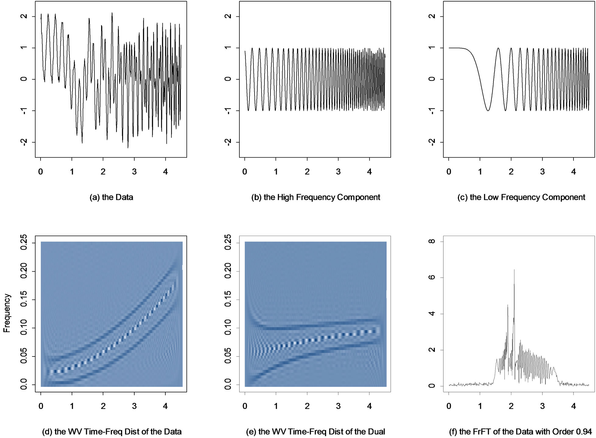
Figure 5. (a) A realization of Example 4.1; (b) and (c) The two actual frequency components; (d) and (e) The Wigner-Ville time-frequency distributions of the data and the dual; (f) The output of the FrFT with order 0.94 to the data.
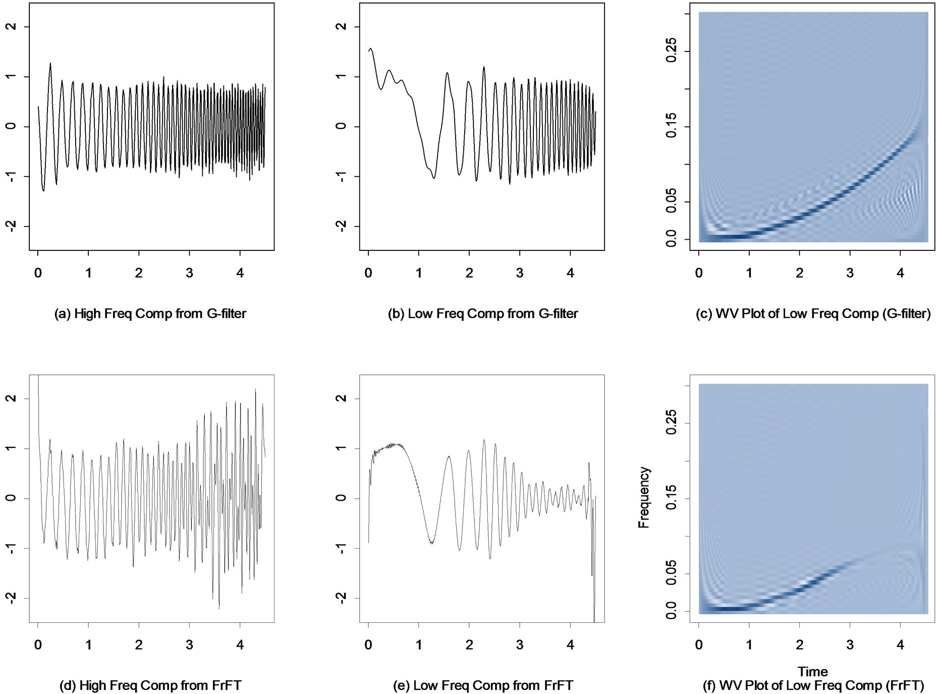
Figure 6. (a) and (b) The two recovered components from the G-filter; (c) The Wigner-Ville time-frequency distribution of the recovered low frequency component from the G-filter; (d) and (e) The two recovered components from the FrFT; (f) The Wigner-Ville time-frequency distribution of the recovered low frequency component from the FrFT.
the outputs of the FrFT show a large spike or an approximate Dirac delta function (Figure 5(f)). Applying the FrFT filtering procedure with order 0.94, we obtain an approximation of the high frequency component. Subtracting it from the original data, we obtain an estimate of the other component. The results are given in Figures 6(d) and (e).
The results in Figure 6 show that the G-filter has successfully recovered both components, while the FrFT recovered the front half of the components (up to time 2.5), but failed afterwards. The Wigner-Ville time-frequency distribution of the filtered low frequency component from the FrFT method (Figure 6(f)) shows that the frequency behavior of this filtered component is very close to linear, indicating that the FrFT has extracted a linear chirp piece rather than the whole quadratic chirp signal. This is not surprising since the FrFT is mainly designed for the linear chirp. There is no order at which the FrFT can produce a Dirac delta function for the quadratic chirp signals as illustrated in this example. The G-filter used a Box-Cox time-deformation function (tλ –1)/λ with λ = 2.7 to deform the phase function of the quadratic chirp signal and thus changed the frequency behavior of the two components so that the frequencies of the components do not overlap anymore. This example shows that the G-filter does not necessarily need to deform the time scale based on the exact frequency structure. Also, this example illustrates the flexibility of the G-filter to filter a wide variety of TVF signals. This flexibility is based on the fact that a wide variety of TVF behaviors, e.g. high order chirp signals, such as quadratic or cubic chirps, can be analyzed using the G(λ) time deformation.
Example 4.2: Consider the process
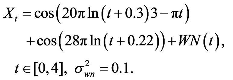
This is a process consisting of two M-stationary components (Gray, et al. (2005) [5]), whose frequency behavior changes like 1/t. A realization of this process and the corresponding Wigner-Ville time-frequency distribution are given in Figures 7(a) and (d). The change in frequency behavior is even further from linearity than that of the quadratic chirps. Clearly, application of the traditional filter will not be effective in separating the two components.
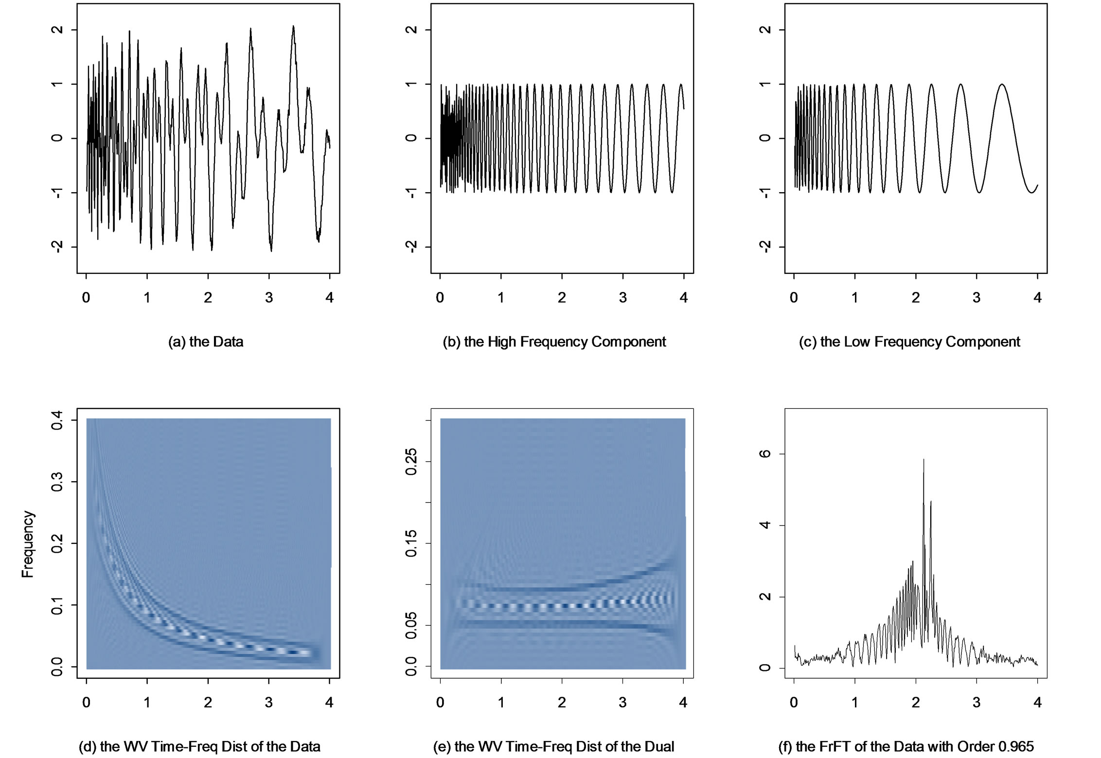
Figure 7. (a) A realization of Example 4.2; (b) and (c) The two actual frequency components; (d) and (e) The Wigner-Ville time-frequency distributions of the data and the dual; (f) The output of the FrFT with order 0.965 to the data.
Using the same technique as in previous example, a G(λ) model with λ = –0.4 and offset = 47 is chosen by GWS to apply the time deformation method for filtering. The two recovered components from the G-filter are given in Figures 8(a) and (b). For the FrFT, at order a = 0.965, the FrFT transforms the process into an output with a large spike (Figure 7(f)). Applying the FrFT with this order produces the outputs as shown in Figures 8(d) and (e). The G-filter has successfully recovered both components, while the FrFT partially filtered out each component as in the previous example. It extracted the signal after time 1.3, but failed before time 1.3. The Wigner-Ville time-frequency distribution of the filtered low frequency component (Figure 8(f)) shows that the FrFT only filtered out a linear chirp type piece, where the frequency change is close to linear.
Note that even a windowing approaching using the FrFT will not be successful because of the sharp frequency change. The data are split into two parts at time 1.3. Figure 9(a) gives the result of the FrFT procedure on the piece before time 1.3. The FrFT still cannot fully filter out the component due to the strong non-linear frequency behavior of this piece of data.
In this example, the phase function of each component is the log function. The G-filter used a Box-Cox time deformation G(–0.4) to transform the data with overlapping frequency behavior into a dual where the frequencies are relatively stable and are non-overlapping (Figures 7(d) and (e)). Here the time-deformation function is not the same as the phase function of the actual signals, suggesting that several different λ values would have produced transformed data on which the frequencies could be separated.
5. Conclusions
The traditional linear filters generally fail to extract components from the non-stationary process with time
Figure 8. (a) and (b) The two recovered components from the G-filter; (c) The Wigner-Ville time-frequency distribution of the recovered low frequency component from the G-filter; (d) and (e) The two recovered components from the FrFT; (f) The Wigner-Ville time-frequency distribution of the recovered low frequency component from the FrFT.

Figure 9. (a) The recovered low frequency component (0:1.3) from the FrFT; (b) The Wigner-Ville time-frequency distribution of this recovered component; (c) The corresponding residuals.
varying frequency behavior. In this paper, we discussed two methods which can be used to filter multi-component non-stationary process: The G-filter and the FrFT method. The G-filter transforms the frequency behavior of the data by deforming the time scale. If viewed from the frequency domain, the G-filter applies a cut-off frequency function according to the frequency behavior of the data. The FrFT method is a generalization of classical Fourier transform, which has been widely used to filter linear chirp signals.
The two filtering methods are similar in that they both transform the data from the original space, where the component is difficult to extract, into a new space where the component can be extracted by available techniques. The original components are then recovered after these filtered components are transformed back into the original space. In the FrFT, the new space is obtained by applying the FrFT with an appropriate order and a masking technique is used to filter out the component in this space. In the G-filter, the new (dual) space is obtained by applying the time-deformation method with an appropriate time deformation function, and a traditional linear filtering technique is used in the dual space to extract each component.
As discussed previously, the FrFT is designed for the linear chirps. As a result, the power of this method closely depends on the underlying frequency structure of the component, i.e. whether its frequency changes linearly with time. If not, the FrFT cannot produce a transformation where a Dirac delta function can be closely approximated and thus can not fully extract the component. For the G-filter, it is not necessary that the component has to be of any particular type. A group of timedeformation functions such as the Box-Cox or G(λ) time-deformation functions have been developed and can be used to either approximate the phase functions of components and thus transform the components into stationary or deformation the phase functions to change the frequency behavior of the data so that the frequency of dual components does not overlap. In conclusion, the G-filter can be used to filter a broad range of components beyond linear chirps, quadratic chirps, etc. The dependence on the exact frequency structure of the component is less stringent in this method, which gives it more flexibility and power over the filtering methods depending on the exact frequency behavior of the data such as the FrFT method.
Finally, we point out that in this research, we used the Butterworth filter to extract components in the dual space, but the G-filtering approach can be incorporated with any other appropriate traditional linear filters. Also, even though in the simulation examples, we used data whose components can each be explicitly written as sinusoidal functions, the G-filter can be applied to any type of stochastic processes where the individual component’s mathematical form may not be explicitly written such as the AR-chirp processes (Liu (2004) [7] and Robertson, et al. (2010) [8]).
REFERENCES
- A. Papoulis, “Probability, Random Variables, and Stochastic Processes,” McGraw-Hill, New York, 1965.
- R. H. Shumway and D. S. Stoffer, “Time Series Analysis and Its Applications,” Springer, New York, 2000.
- S. Butterworth, “On the Theory of Filter Amplifiers,” Experimental Wireless and the Wireless Engineer, Vol. 7, 1930, pp. 536-541.
- M. Xu, K. B. Cohlmia, W. A. Woodward and H. L. Gray, “G-Filtering Nonstationary Time Series,” Journal of Probability and Statistics, Vol. 2012, 2012, Article ID: 738636. doi:10.1155/2012/738636
- H. L. Gray, C. C. Vijverberg and W. A. Woodward, “Nonstationary Data Analysis by Time Deformation,” Communication in Statistics-Theory and Methods, Vol. 34, No. 1, 2005, pp. 163-192. doi:10.1081/STA-200045869
- H. Jiang, H. L. Gray and W. A. Woodward, “TimeFrequency Analysis—G(λ) stationary Processes,” Computational Statistics & Data Analysis, Vol. 51, No. 3, 2006, pp. 1997-2028. doi:10.1016/j.csda.2005.12.011
- L. Liu, “Spectral Analysis with Time-Varying Frequency,” Ph.D. Dissertation, Southern Methodist University, Boaz Lane Dallas, 2004. doi:10.1016/j.jspi.2010.04.033
- S. D. Robertson, H. L. Gray and W. A. Woodward, “The Generalized Linear Chirp Process,” Journal of Statistical Planning and Inference, Vol. 140, No. 12, 2010, pp. 3676- 3687.
- B. Boashash, “Time Frequency Analysis,” Elsevier, Oxford, 2003.
- R. G. Baraniuk and D. L. Jones, “Unitary Equivalence: A New Twist on Signal Processing,” IEEE Transactions on Signal Processing, Vol. 43, No. 11, 1995, pp. 2269-2282. doi:10.1109/78.469861
- M. Xu, “Filtering Non-Stationary Time Series by Time Deformation,” Ph.D. Dissertation, Southern Methodist University, Dallas, 2004.
- H. M. Ozaktas, O. Arikan, M. A. Kutay and G. Bozdagt, “Digital Computation of the Fractional Fourier Transform,” IEEE Transactions on Signal Processing, Vol. 44, No. 9, 1996, pp. 2141-2150. doi:10.1109/78.536672
- C. Capus and K. Brown, “Short-Time Fractional Fourier Methods for the Time-Frequency Representation of Chirp Signals,” Journal of Acoustical Society of America, Vol. 113, No. 6, 2003, pp. 3253-3263. doi:10.1121/1.1570434
- H. M. Ozaktas, Z. Zalevsky and M. A. Kutay, “The Fractional Fourier Transform,” John Willey & Sons, Ltd., New York, 2000.