Journal of Signal and Information Processing
Vol. 3 No. 1 (2012) , Article ID: 17654 , 12 pages DOI:10.4236/jsip.2012.31008
Using Two Levels DWT with Limited Sequential Search Algorithm for Image Compression
![]()
Software Engineering Department, Technical College, Kirkuk, Iraq.
Email: mamadmmx76@yahoo.com
Received November 10th, 2011; revised December 12th, 2011; accepted December 21st, 2011
Keywords: DWT; DCT; Minimize-Matrix-Size-Algorithm; LSS-Algorithm; Eliminate Zeros and Store Data
ABSTRACT
In this paper introduce new idea for image compression based on the two levels DWT. The low-frequency sub-band is minimized by using DCT with the Minimize-Matrix-Size-Algorithm, which is converting the AC-coefficients into array contains stream of real values, and then store the DC-coefficients are stored in a column called DC-Column. DC-Column is transformed by one-dimensional DCT to be converted into T-Matrix, then T-Matrix compressed by RLE and arithmetic coding. While the high frequency sub-bands are compressed by the technique; Eliminate Zeros and Store Data (EZSD). This technique eliminates each 8 × 8 sub-matrix contains zeros from the high frequencies sub-bands, in another hands store nonzero data in an array. The results of our compression algorithm compared with JPEG2000 by using four different gray level images.
1. Introduction
Digital representation of image has created the need for efficient compression algorithms that will reduce the storage space and the associated channel bandwidth for the transmission of images. Wavelet transforms have become more and more popular in the last decade in the field of image compression [1]. They have an advantage over the block-based transforms such as Discrete Cosine Transform (DCT) which exhibits blocking artifact. Wavelets with compact support provide a versatile alternative to DCT [2]. The groundbreaking single-wavelet examples provided multiresolution function-approximation bases formed by translations and dilations of a single approximation functions and detail functions. In the last years multi-wavelets, which consist of more than one wavelet have attracted many researchers [3]. Certain properties of wavelets such as orthogonally, compact support, linear phase, and high approximation/vanishing moments of the basis function, are found to be useful in image compression applications. Unfortunately, the wavelets can never possess all the above mentioned properties simultaneously [4]. To overcome these drawbacks, more than one scaling function and mother wavelet function need to be used. Multi-wavelets posses more than one scaling function offer the possibility of superior performance and high degree of freedom for image processing applications, compared with scalar wavelets. Multi-wavelets can achieve better level of performance than scalar wavelets with similar computational complexity [5]. In the case of nonlinear approximation with multi-wavelet basis, the multiwavelet coefficients are effectively “reordered” according to how significant they are in reducing the approximation error [6]. The JPEG2000 is a new image compression standard, recently, introduced by Joint Picture Experts Group [7]. In addition to its improved compression ability, JPEG2000 provides many features which are of high importance to many applications in which the quality and performance criteria are crucial, such applications are scanning, remote sensing, recognition, medical imaging [8]. Comparative test results have shown that the JPEG2000 is superior to existing still image compression standards [9]. A review paper as well as comparative works with the existing compression standards can be found in the literature. JPEG2000 start with discrete wavelet transform to the source image data. The coefficients obtained from the wavelet transform are then quantized and entropy coded, before forming the output bit stream. JPEG2000 standard supports both lossy and lossless compression. This depends on the wavelet transform and the quantization applied [10].
This research introduces a new idea for image compression depending on two transformations with MinimizeMatrix-Size algorithm and using LSS-Algorithm for decoding.
2. Proposed Compression Algorithm
Our image compression algorithm uses two transformations. First transformation is two levels DWT, converts the images into seven sub-bands, and the second transformation is two dimensional DCT applied on each “2 × 2” block of data from low-frequency sub-band “LL2”. The DCT is very important for our approach sharing with DWT for obtains more high-frequencies domains. DCT plays main role for converting sub-band “LL2” into DCcoefficients and AC-coefficients, DC-coefficients stored in a column called DC-Column, while AC-coefficients are stored in the AC-Matrix, and then applied MinimizeMatrix-Size Algorithm on the AC-Matrix to convert ACcoefficients into array, as shown in Figure 1.
2.1. Using Discrete Wavelet Transform (DWT)
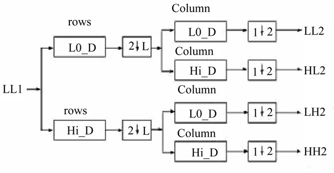
Wavelet transform has the capability to offer some information on frequency-time domain simultaneously. In this transform, time domain is passed through low-pass and high-pass filters to extract low and high frequencies respectively. This process is repeated for several times and each time a section of the signal is drawn out. DWT analysis divides signal into two classes (i.e. Approximation and Detail) by signal decomposition for various frequency bands and scales [11]. DWT utilizes two function sets: scaling and wavelet which associate with low and high pass filters orderly. Such a decomposition manner bisects time separability. In other words, only half of the samples in a signal are sufficient to represent the whole signal, doubling the frequency separability. Figure 2 shows two level decomposition the “Lena” image.
The wavelet decomposition has some important fea-
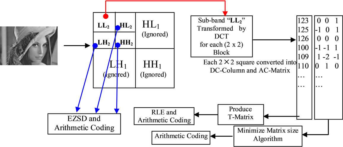
Figure 1. Applied Minimize-Matrix-Size algorithm on the LL2 sub-band.
 (a)
(a) (b)
(b)
Figure 2. (a) First level decomposition for “Lena” image; (b) Second level decomposition “Lena” image.
tures; many of the coefficients for the high-frequency components (LH, HL and HH) are zero or insignificant [12]. This reflects the fact that the much of the important information is in “LL” sub-band. The DWT is a good choice of transform accomplishes a de-correlation for the pixels, while simultaneously providing a representation in which most of the energy is usually restricted to a few coefficients [13], while other sub-bands (i.e. LH1, HL1 and HH1) are ignored. This is the key for achieving a high compression ratio. The Daubechies Wavelet Transform family has ability to reconstructs images, by using just LL1 without need for other high-frequencies. But this leads for obtains less image quality.
2.2. Using Discrete Cosine Transform (DCT)
DCT is the second transformation is used in this research, which is applies on each “2 × 2” block from “LL2” sub-band as show in Figure 3.
DCT produce DC value and AC coefficients. Each DC value is stored in the DC-Column, and the other three AC coefficients are stored in the AC-Matrix.
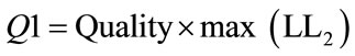
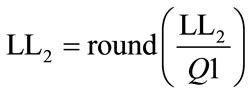
2.2.1. Quantization Level1
In the above Figure 3, “Quantization level1” is used to reduce size of the data for LL2, by select the ratio of maximum value for LL2 as shown in the following equations:
 (1)
(1)
 (2)
(2)
“Quality” value is used in Equation (1), affects in the image quality. For example “Quality = 0.005”, this means compute 0.5% from maximum value in LL2 to be divided by all values in LL2. This process helps the LL2 values to be more converging (i.e. more correlated). In another hands this quantization process leads to obtains low image quality, if the Quality > 1%.
2.2.2. Quantization Level2
Each “2 × 2” coefficients from LL2 is transformed by DCT and then divided by “Q2”, using matrix-dot-division. This process removes insignificant coefficients and increasing the zeros in the transformed LL2. The “Q2” can be computed as follows [4]:
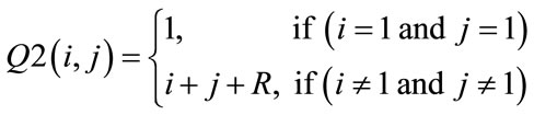 (3)
(3)
2.2.3. Using Two Dimensional DCT
The energy in the transformed coefficients is concentrated about the top-left corner of the matrix of coefficients. The top-left coefficients correspond to low fre-
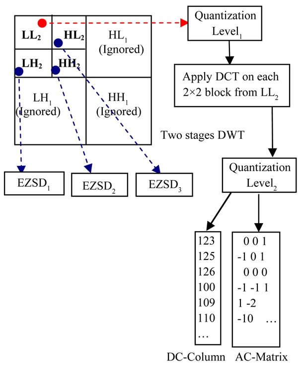
Figure 3. LL2 sub-band quantized and transformed by DCT for each 2 × 2 blocks.
quencies: there is a “peak” in energy in this area and the coefficients values rapidly decrease to the bottom right of the matrix, which means the higher-frequency coefficients [3].
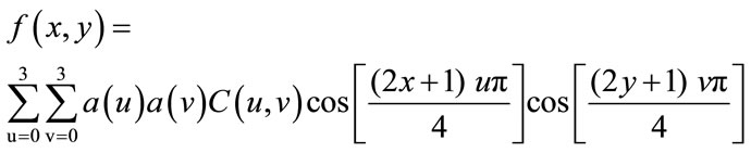
The DCT coefficients are de-correlated, which means that many of the coefficients with small values can be discarded without significantly affecting image quality. A compact matrix of de-correlated coefficients can be compress much more efficiently than a matrix of highly correlated image pixels [4]. The following equations illustrated DCT and Inverse DCT function for two-dimensional matrices “2 × 2”:
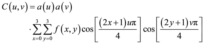 (4)
(4)
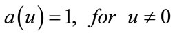
where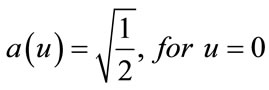 ,
, 
 (5)
(5)
One of the key differences between the applications of the Discrete Wavelet transformation (DWT) and Discrete Cosine transformation (DCT) is; the DWT typically apply to an image as a one block or a large rectangular region of the image, while for the small block size using DCT. The DCT becomes increasingly complicated to calculate for the larger block sizes, for this reason in this paper used “2 × 2” block to be transformed by DCT, whereas a DWT will be more efficiently applied to the complete images and produce good compression ratio.
2.3. Apply Minimize-Matrix-Size Algorithm
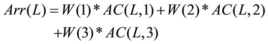
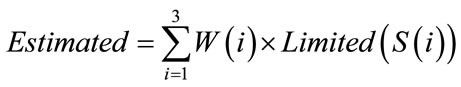
The DWT and DCT it’s used for increasing number of the high-frequency coefficients, but this is not enough in our approach, for this reason in this research introduces a new algorithm for minimizing the size of AC-Matrix into array. This algorithm based on the Random-WeightsValues. The following equation represents converting AC-Matrix into array:
 (6)
(6)
Note: “AC” is represents AC-Matrix.
L = 1, 2, 3,··· Column size of AC-Matrix.
The “W” in Equation (6) is represents RandomWeights-Values, generated by random function in MATLAB language, the “W” values between {0···1}, for example: W = {0.1, 0.65, 0.423}. The Random-WeightsValues are multiply with each row from AC-Matrix, to produce single floating point value “Arr”, this idea it’s similar to the neural network equations. The neural networks equations; multiplies the updated weights values with input neurons to produce single output neuron [14]. Minimize-Matrix-Size Algorithm is shown in the following List 1:
Before apply the Minimize-Matrix-Size algorithm, our compression algorithm computes the probability of the AC-Matrix. These probabilities are called Limited-Data, which is used later in decompression algorithm, the Limited-Data stored in the header for compressed file. Because these data uncompressible.
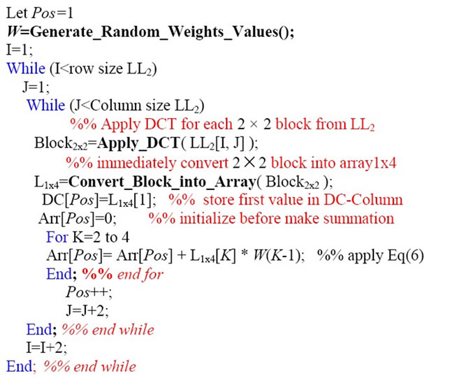
List 1. Minimize-Matrix-Size algorithm.
Figure 4 illustrates probability of data for a matrix.
The final step in this section is; Arithmetic coding, which takes stream of data and convert it into single floating point value. These output values in the range less than one and greater than zero, when decoded this value getting exact stream of data. The arithmetic coding need to compute the probability of all data and assign range for each data, the range value consist from Low and High value [3,4].
2.4. T-Matrix Coding
The DC-Column contains integer values, these values are obtained from pervious section (See Section 2.2). The arithmetic coding unable to compress this column, because these values are correlated, for this reason DCColumn partitioned into 128-parts, and each partition is transformed by DCT (See Equation (1)) as a one-dimensional array by using u = 0 and x = 0 in Equation (1) to be one-dimensional DCT and then using quantization process for each row, as shown in the following equation:
 (7)
(7)
Note: n= 2, 3, ···, 128.
The initial value of Q(1) = 12.8.
The first value in above Equation (7) is Q(1) = 12.8, because the length of each row is 128. Each 128 values are transformed and stored as a row in the matrix called Transformed-Matrix (T-Matrix). This part of our compression algorithm it’s look like JPEG technique, as shown in Figure 5. The idea for using T-Matrix, this is because we need to increase number of zeros or insignificant and makes values more de-correlated, this process increases compression ratio. Each row from T-Matrix consists of; DC value and stream of AC coefficients, now we need to scan T-Matrix column-by-column for converting it into one-dimensional array, and then compress it by Run Length Encoding (RLE) and arithmetic coding.
RLE it counts the repeated coefficients, and then refers to the repeated coefficients by a value, this process reduce the length of the repeated data, then applying the arithmetic coding to convert these reduced data into bits. For more information about RLE and Arithmetic coding is in [3,4].
2.5. Applied Eliminate Zeros and Store Data (EZSD)
This technique is used in this research to eliminate block of zeros, and store block of nonzero data in an array. This technique is very useful for reducing the size of the high-frequencies sub-bands (i.e. HL2, LH2 and HH2) or the matrices which is contains more zeros, EZSD applied on each sub-band independently. Before applying EZSD
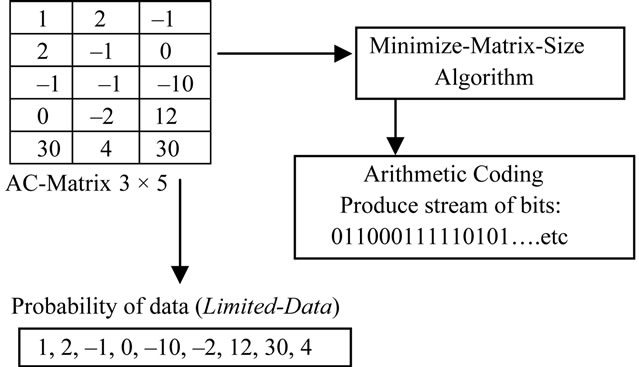
Figure 4. Illustrates probability of data (limited-data) for the AC-Matrix 3 × 5.
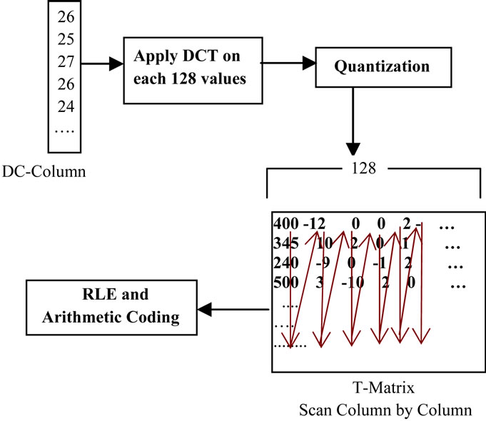
Figure 5. T-Matrix coding technique.
algorithm each high-frequency sub-band (i.e. HL2, LH2 and HH2) is quantized with Quantization level1 (See Equation (2)), with Quality value >= 0.01.
This is because to removing insignificant coefficients and increasing number of zeros.
EZSD algorithm starts to partition the high-frequencies sub-bands into non-overlapped 8 × 8 blocks, and then starts to search for nonzero block (i.e. search for any data inside a block). If the block contains any data, this block will be stored in the array called Reduced Array, and the position for that block is stored in new array called Position. If the block contains just zeros, this block will be ignored, and jump to the next block, the algorithm summarized in List 2. Figure 6 shows just LH2 high-frequency sub-band partitioned into 8x8 block and coded by EZSD Algorithm.
The EZSD algorithm applied on each high-frequency sub-band (See Figure 3). The problem of EZSD technique is; the reduced array still has some of zeros, this is because some blocks contain few data in some locations, while others are zeros. This problem has been solved by eliminating the zeros from reduced array. Figure 7 illus-
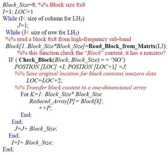
List 2. EZSD algorithm.
trates eliminating zeros from the Reduced Array. The idea for eliminating just eight zeros or less from “Reduced Array”, this is because to repeat counts of zeros. For the above example “0, 8” repeated 4 times, “0, 1” and “0, 4” are repeated 2 times, this process increases compression ratio with arithmetic coding.
3. Our Decompression Algorithm
Our decompression algorithm represents inverse of our compression algorithm, which is consist of four phases illustrated in the following points:
1) First phase; decoding all high-frequencies domains for the second level of DWT (i.e. HL2, LH2 and HH2).
2) Second phase; decoding DC-Column.
3) Third phase; decoding AC-Matrix by using LSSAlgorithm.
4) Fourth phase; combine DC-Column with AC-Matrix to reconstruct approximately LL2 coefficients, and finally apply inverse DWT to get decompressed image.
3.1. Decode High-Frequency Sub-Band
This section discusses the high-frequencies are decoded, by expansion for reduced data (See Section 2.5). The expansion is meaning, looking for a zero followed by a number, this number is count’s zero, the algorithm repeat zeros according to the number in a new array called Expanded Array. Finally replace each 64-data as a block in an empty matrix, according to it is position in the matrix (See List 2). This decoding algorithm is applied to each reduced array for each sub-band independently. Figure 8 illustrates just LH2 decoding.
3.2. Decode DC-Column
Run Length Decoding (RLD) and Arithmetic decoding,
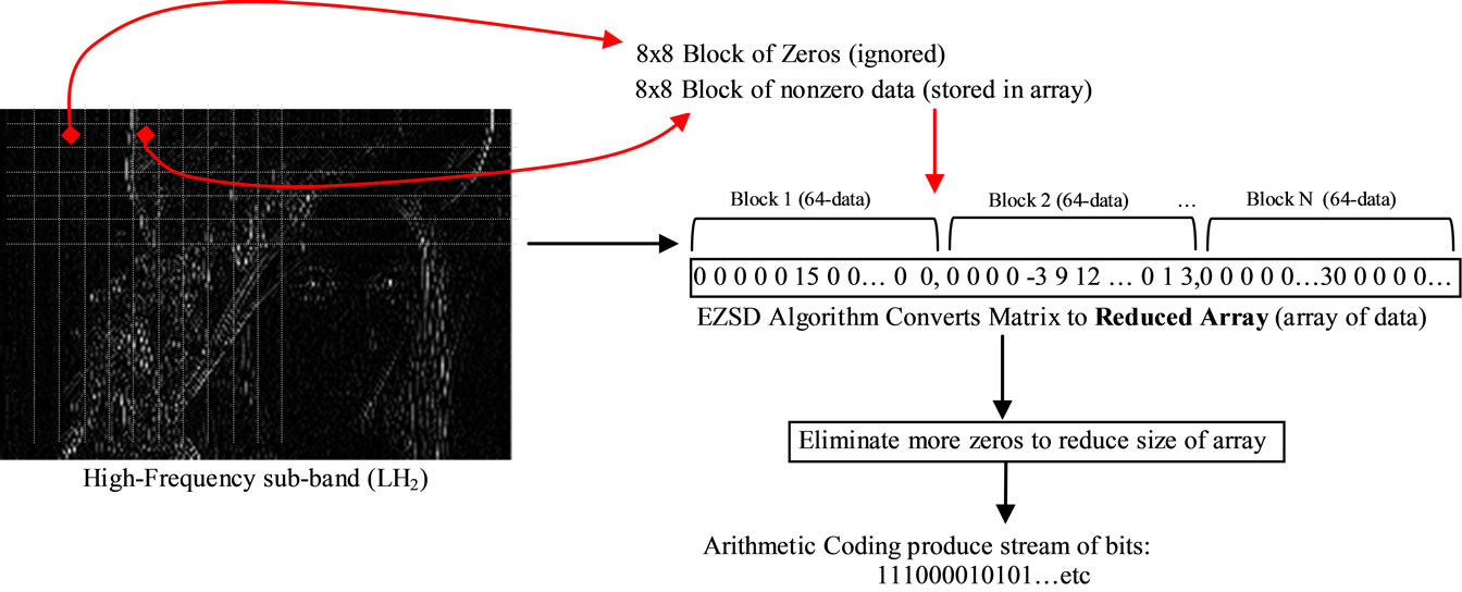
Figure 6. EZSD algorithm applied on LH2 sub-band.
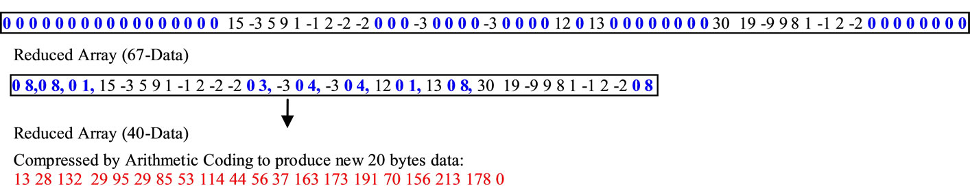
Figure 7. Illustrates eliminating more zeros from reduced array.
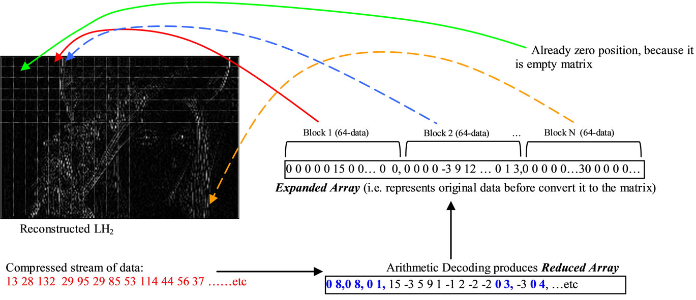
Figure 8. Illustrates first phase decoding for LH2 reconstructed.
produced one-dimensional-array contains the original data for the T-Matrix. This array reads element-byelement, and placed in the columns of the T-Matrix.
After generates the T-Matrix, applied Inverse Quantization, It is dot-multiplication of the row coefficients with “Q(n)” (See Equaton (7)), then one-dimensional inverse DCT applied on each row to produce 128-values (See Equation (5)), this process will continues until all rows are completes. Figure 9 illustrates DC-Column decoding.
3.3. Limited Sequential Search Algorithm Decoding
This algorithm is used for reconstruct AC-Matrix, by using minimized data (See Equation (6)), and Random-Weights-
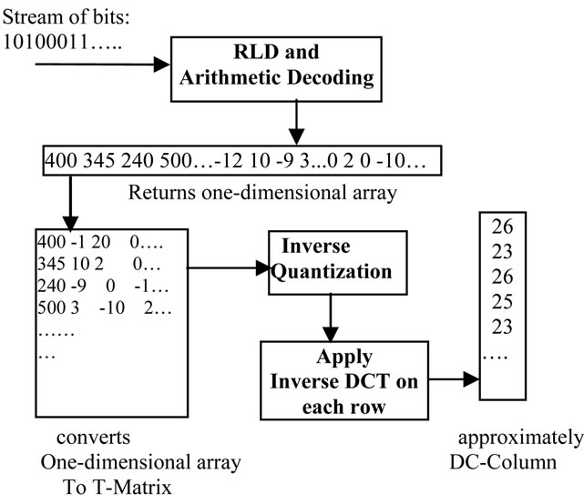
Figure 9. Second phase for our decompression algorithm “Decoding DC-Column”.
Values. This algorithm is depends on the pointers for finding the missed data inside the Limited-Data for ACMatrix. If the Limited-Data is missed or destroyed, the AC-Matrix couldn’t return back. Figure 10 shows ACMatrix decoded by LSS-Algorithm.
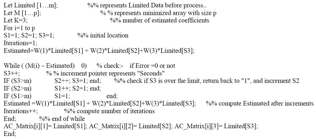
The LSS-Algorithm is designed for finding missing data inside a Limited-Data, by using three pointers. These pointers are refers to index in the Limited-Data, the initial value for these pointers are “1” (i.e. first location in a Limited-Data). These three pointers are called S1, S2 and S3; these pointers increment by one at each iteration (i.e. these three pointers work as a digital clock, where S1, S2 and S3 represent hour, minutes and seconds respectively). To illustrate LSS-Algorithm assume we have the following matrix 2 * 3:
EXAMPLE:
30 | 1 | 0 |
19 | 1 | 1 |
In the above example the matrix will compress by using Minimize-Matrix-Size algorithm to produce minimized data; M(1) = 3.65 and M(2) = 2.973, the LimitedData = {30,19,1,0}. Now the LSS-Algorithm will estimates the matrix 2*3 values, by using the Limited-Data and the Random-Weight-Values = {0.1, 0.65, and 0.423}. The first step in our decompression algorithm, assign S1 = S2 = S3 = 1, then compute the result by the following equation:
 (8)
(8)
W: generated weights.
Limited: Limited Data.
S(i): pointers 1,2 and 3.
LSS-Algorithm computes “Estimated” at each iteration,

Figure 10. Third phase of our decompression algorithm “Decoding AC-Matrix”.
and compare it with “M(i)”. If it is zero, the estimated values are FOUND at locations= {S1, S2 and S3}. If not equal to zero, the algorithm will continue to find the original values inside the limited-data. The List 3 illustrates LSS-Algorithm, and Figure 11 illustrates LSS-Algorithm estimates matrix values for the above example.
At the fourth phase; our decompression algorithm combines DC-Column and AC-Matrix, and then apply inverse DCT (See Equation (5)) to reconstructs LL2 sub-band, then applying first level inverse DWT on LL2, HL2, LH2 and HH2 to produce approximately LL1. The second level inverse DWT applied on LL1 and other subbands are zeros to reconstructs approximately original image.
4. Computer Results
Our compression and decompression algorithm tested on the three gray level images “Lena”, “X-ray” and “Girl”. These images are executed on Microprocessor AMD Athalon ~2.1 GHz with 3G RAM and using MATLAB R2008a programming language under the operating system Windows-7 (32 bit). Figure 12 shows the three original images used for test. Our compression algorithm parameters are summarized in the following; 1) Using two level Daubechies DWT “db5”. 2) High-frequencies subbands (i.e. HL1, LH1 and HH1) are zeros (ignored). 3) LL2 quantized by Quantization level1 (See Equation (2)) with Quality = 0.005. 4) Applied two dimensional DCT for each 2 × 2 block and Quantization Level2 (See Equation (3)) with R = 5. 5) AC-Matrix compressed by using Minimized-Matrix-Size Algorithm with W = {0.1, 0.65,
List 3. LSS-Algorithm.
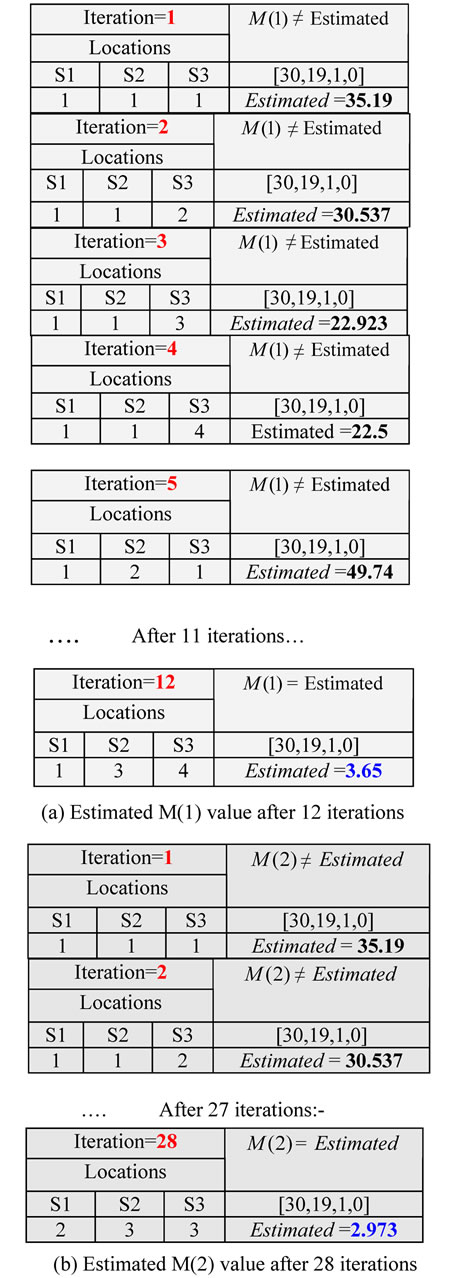
Figure 11. (a,b) LSS-Algorithm finds estimated for the matrix 2 * 3.
 (a)
(a) (b)
(b) (c)
(c)
Figure 12. Original images used for test by our approach. (a) Lena image, size = 420 Kbytes, dimension (795 × 539); (b) X-ray image, size = 588 Kbytes, dimension (997 × 602); (c) Girl image, size= 489 Kbytes, dimension (830 × 601).
0.423}. 6) High-frequencies (HL2, LH2 and HH2) divided into 8 × 8 blocks, and then compressed by using EZSD algorithm.
Table 1 shows the results of our compression algorithm, for each image with different use of Quality parameter.
Our decompression algorithm illustrated in Section 3, used for decoding the compressed image data, Table 2 shows PSNR for the decoded images and time execution for LSS-Algorithm used to reconstructs AC-Matrix for each image.
PSNR it is used in Table 2, refers to image quality mathematically, PSNR it is a very popular quality measure, can be calculates very easily between the decom-
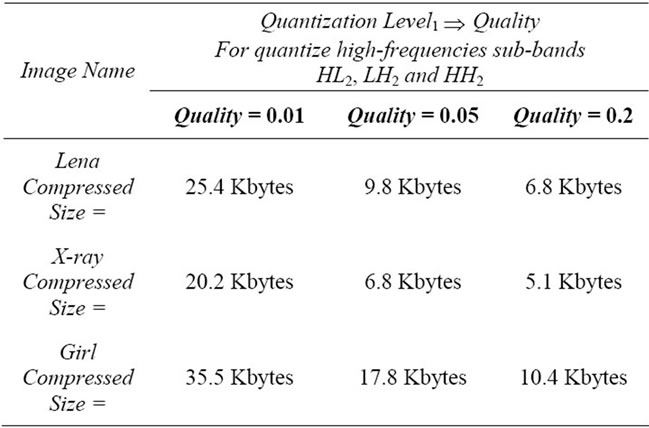
Table 1. Our compression algorithm results.
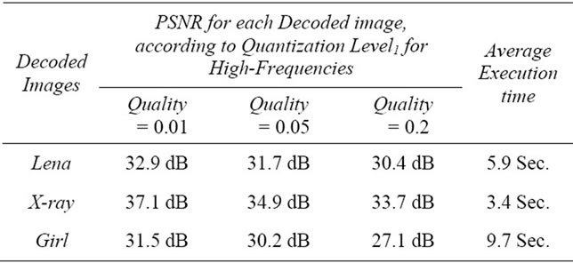
Table 2. PSNR and LSS-Algorithm execution time for decode images.
pressed image and its original image [3,4,8]. Our approach is compared with JPEG2000, which is represents one of the best image compression techniques. JPEG2000 consists of; three main phases illustrated in the following steps:
Discrete Wavelet Transform (DWT): Tile components are decomposed into different decomposition levels using wavelet transform, which improves JPEG2000’s compression efficiency due to its good energy compaction and the ability to de-correlate the image across a larger scale [12].
Quantization: In this step, the coefficients obtained from the wavelet transform are reduced in precision. This process is lossy, unless the coefficients are real and obtained by reversible bi-orthogonal 5/3 wavelet transform.
The quantizer indices corresponding to the quantized wavelet coefficients in each sub-band are entropy encoded to create the compressed bit-stream. The quantized coefficients in a code-block are bit-plane encoded independently from all other code-blocks when creating an embedded bit stream [13].
Arithmetic Coding: Arithmetic coding uses a fundamentally different approach from Huffman coding in such way that the entire sequence of source symbols is mapped into a single very long codeword. This codeword is built by recursive interval partitioning using the symbol probabilities. In this research we used ACDSee applications for save images as JPEG2000 format; an ACDSee application has many options to save the images as JPEG2000 format. The most option is using; “Quality”. If the image quality is increased the compression ratio is decreased and vice versa. The comparison between JPEG2000 and our approach is based on image quality, when JPEG2000 compressed image size it is equivalent to compressed size by our approach.
Table 3 shows PSNR and compressed size for each image by using JPEG2000 and our approach, and Figure 13, Figure 14 and Figure 15 show decoded images by our approach compared with JPEG2000 according to the quality factor.
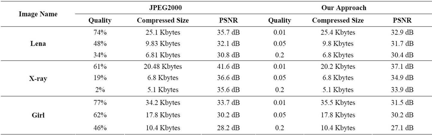
Table 3. Comparison between JPEG2000 and our approach.
 (a)
(a) (b)
(b)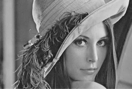 (c)
(c) (d)
(d) (e)
(e) (f)
(f)
Figure 13. Decoded “Lena” image with different quality values by our approach and JPEG2000. (a) Decoded by our approach with Quality = 0.01, PSNR = 32.9 dB; (b) Decoded by JPEG2000 with Quality = 74%, PSNR = 35.7; (c) Decoded by our approach with Quality = 0.05, PSNR = 31.7 dB; (d) Decoded by JPEG2000 with Quality = 48%, PSNR = 32.1 dB; (e) Decoded by our approach with Quality = 0.2, PSNR = 30.4 dB; (f) Decoded by JPEG2000 with Quality = 34%, PSNR = 30.8 dB.
 (a)
(a) (b)
(b) (c)
(c) (d)
(d) (e)
(e)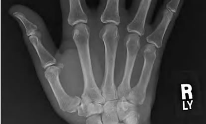 (f)
(f)
Figure 14. Decoded “X-ray” image with different quality values by our approach and JPEG2000. (a) Decoded by our approach with Quality = 0.01, PSNR = 37.1 dB; (b) Decoded by JPEG2000 with Quality = 61%, PSNR = 41.6 dB; (c) Decoded by our approach with Quality = 0.05, PSNR = 34.9 dB; (d) Decoded by JPEG2000 with Quality = 19%, PSNR = 36.6 dB; (e) Decoded by our approach with Quality = 0.2, PSNR = 33.9 dB; (f) Decoded by JPEG2000 with Quality = 2%, PSNR = 35.6 dB.
 (a)
(a) (b)
(b) (c)
(c) (d)
(d) (e)
(e) (f)
(f)
Figure 15. Decoded “Girl” image with different quality values by our approach and JPEG2000. (a) Decoded by our approach with Quality = 0.01, PSNR = 31.5 dB; (b) Decoded by JPEG2000 with Quality = 77%, PSNR = 33.7 dB; (c) Decoded by our approach with Quality = 0.05, PSNR = 30.2 dB; (d) Decoded by JPEG2000 with Quality = 62%, PSNR = 30.2 dB; (e) Decoded by our approach with Quality = 0.2, PSNR = 27.1 dB; (f) Decoded by JPEG2000 with Quality = 46%, PSNR = 28.2 dB.
5. Conclusions
This research introduces a new image compression and decompression algorithms, based on the two important transformations (DCT and DWT) with Minimize-MatrixSize algorithm and LSS-Algorithm. This research has some advantages illustrated in the following steps:
1) Using two transformations, this helped our compression algorithm to increases number of high-frequency coefficients, and leads to increases compression ratio.
2) Used two levels quantization for LL2 sub-band and one level quantization for high-frequencies sub-bands at second level DWT. This process increasing number of zeros in the matrix.
3) Minimize-Matrix-Size algorithm it is used to converts three coefficients from AC-Matrix, into single floating point value. This process increases compression ratio, and in another hand keep the quality of the highfrequency coefficients.
4) The properties of the Daubechies DWT (db5) helps our approach to obtain higher compression ratio, this is because the high-frequencies for first level is ignored in our approaches. This is because the Daubechies DWT family has the ability to zooming-in, and does not necessarily needs for the high-frequencies sub-bands.
5) LSS-Algorithm is represents the core of our decompression algorithm, which converts the one-dimensional array into the AC-Matrix. This algorithm is depending on the Random-Weights-Values. LSS-Algorithm finds solution as faster as possible with three pointers (See time execution Table 2).
6) Limited-Data is represents the key of the decompressed image, this is represents security for the decompressed images, if the users needs to hide the keys.
7) Our approach gives good visual image quality, more than JPEG2000. This is because our approach removes the blurring and an artifact that caused by Multi-level DWT and quantization in JPEG2000 (See Figures 13, 14, 15).
8) The EZSD algorithm used in this research used to removes a lot of zeros, and at same time converts a highfrequency sub-band to array, this process increases compression ratio.
Also this research has some disadvantages illustrated in the following steps:
1) High-frequencies sub-bands at first level of DWT are ignored, this causes low quality decompressed images (See Table 3).
2) The speed of LSS-Algorithm depends on the LimitData length for an AC-Matrix; this makes our approach slower than JPEG2000.
3) Minimize-Matrix-Size algorithm converts an AC-Matrix to an array contains stream of floating point values. The minimized array coded by arithmetic coding, the header size of the compressed data may be more than 2 Kbytes.
4) If the Limited-Data for the compressed file is lost or damaged, the image couldn’t be decompressed
REFERENCES
- G. Sadashivappa and K. V. S. Ananda Babu, “Performance Analysis of Image Coding Using Wavelets,” IJCSNS International Journal of Computer Science and Network Security, Vol. 8 No. 10, 2008, pp. 144-151.
- A. Al-Haj, “Combined DWT-DCT Digital Image Watermarking,” Journal of Computer Science, Vol. 3, No. 9, 2007, pp. 740-746.
- K. Sayood, “Introduction to Data Compression,” 2nd Edition, Academic Press, San Diego, 2000.
- R. C. Gonzalez and R. E. Woods “Digital Image Processing,” Addison Wesley Publishing Company, Reading, 2001.
- M. Tsai and H. Hung, “DCT and DWT Based Image Watermarking Using Sub Sampling,” Proceeding of the Fourth International Conference on Machine Learning and Cybern, Guangzhou, 18-21 August 2005, pp. 5308- 5313.
- S. Esakkirajan, T. Veerakumar, V. Senthil Murugan and P. Navaneethan, “Image Compression Using Multiwavelet and Multi-Stage Vector Quantization,” International Journal of Signal Processing, Vol. 4, No. 4, 2008. http://www.waset.org/journals/ijice/v4/v4-4-32.pdf
- M. Antonini, M. Barlaud, P. Mathieu and I. Daubechies, “Image Coding Using Wavelet Transform,” IEEE Transactions on Image Processing, Vol. 1, No. 2, 1992, pp. 205-220. doi:10.1109/83.136597
- I. E. G. Richardson, “Video Codec Design,” John Wiley & Sons, New York, 2002. doi:10.1002/0470847832
- T. Acharya and P. S. Tsai. “JPEG2000 Standard for Image Compression: Concepts, Algorithms and VLSI Architectures,” John Wiley & Sons, New York, 2005.
- S. Ktata, K. Ouni and N. Ellouze, “A Novel Compression Algorithm for Electrocardiogram Signals Based on Wavelet Transform and SPIHT,” International Journal of Signal Processing, Vol. 5, No. 4, 2009, pp. 32-37.
- R. Janaki and A. Tamilarasi, “Visually Improved Image Compression by Using Embedded Zero-Tree Wavelet Coding,” IJCSI International Journal of Computer Science Issues, Vol. 8, No. 2, 2011, pp. 593-599.
- S. M. Basha and B. C. Jinaga, “A Robust Image Compression Algorithm Using JPEG 2000 Standard with Golomb Rice Coding,” IJCSNS International Journal of Computer Science and Network Security, Vol. 10, No. 12, 2010, pp. 26-33.
- C. Christopoulos, J. Askelof and M. Larsson, “Efficient Methods for Encoding Regions of Interest in the Upcoming JPEG 2000 Still Image Coding Standard,” IEEE Signal Processing Letters, Vol. 7, No. 9, 2000, pp. 247-249. doi:10.1109/97.863146
- M. M. Siddeq, “Image Restoration Using Perception Neural Network,” Master Thesis, Computer Science Department, University of Technology, Iraq, 2001.